
When designing or evaluating a mineral processing plant, one of the most important questions is not only how much the plant can process when all equipment is operating, but how much it can actually produce over time.
Real plants do not operate continuously under ideal conditions. Feed rates vary, equipment stops, repairs take time, stockpiles fill and empty, and operators respond to changing process conditions. A reliability study helps translate these events into engineering indicators such as operating hours, production losses, plant availability, and bottleneck sensitivity.
In mineral processing, this is especially important because the impact of a failure is rarely limited to the failed equipment itself. A stopped conveyor may interrupt a crusher. A full stockpile may stop upstream equipment. An empty surge bin may starve the grinding circuit. For this reason, reliability must be understood not only at the equipment level, but also at the flowsheet level.

From Equipment Failures to Plant Performance
A processing plant can be viewed as a network of unit operations connected by material streams. Each equipment item may be operating, stopped, under maintenance, waiting for feed, blocked by downstream capacity, or bypassed by an operating strategy.
Traditional reliability calculations often start by asking whether each item is available or unavailable. This is a useful first step, but plant performance also depends on how equipment interacts with the rest of the circuit.
For example, the failure of a feeder upstream of a large stockpile may have little immediate effect on the downstream plant. The same feeder failure without intermediate storage may stop the entire circuit almost immediately. In both cases, the equipment reliability may be the same, but the production impact is different.
This distinction is central to DPSIM reliability studies: equipment failures are modeled together with process dynamics, inventories, operating rules, and flowsheet interactions.
Basic Reliability Indicators
Before analyzing a complete plant, it is useful to understand two basic time-based indicators: MTBF and MTTR.
MTBF – Mean Time Between Failures
MTBF represents the average operating time between failures for a repairable item.
If a pump typically operates for 1,000 hours before failing, its MTBF is approximately 1,000 hours. A higher MTBF means that failures are less frequent. In engineering terms, MTBF is commonly used as an indicator of reliability.
MTBF does not say how long the repair will take. It only describes how often failures are expected to occur.
MTTR – Mean Time to Repair
MTTR represents the average time required to restore the equipment after a failure.
If a conveyor has five failures and the total repair time is 200 hours, the MTTR is 40 hours. A lower MTTR means that the system can recover more quickly after a failure. In engineering terms, MTTR is commonly used as an indicator of maintainability.
MTTR does not say how often the failure occurs. It only describes how long recovery tends to take once a failure has occurred.
Reliability, Availability and Maintainability
Reliability, availability and maintainability are related concepts, but they answer different engineering questions.
- Reliability asks: what is the probability that the equipment will perform its function without failing during a given period?
- Availability asks: what fraction of time is the equipment expected to be ready for operation?
- Maintainability asks: how quickly can the equipment be restored after a failure?
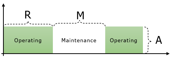
A piece of equipment may be reliable but difficult to repair. Another may fail more often but be restored very quickly. These two cases can lead to different operating behavior and different impacts on plant production.
For a repairable item, a common estimate of inherent availability is:
This equation shows the basic balance between failure frequency and repair duration. Availability improves when failures become less frequent or when repairs become faster.
However, in a mineral processing plant, equipment availability alone does not fully describe production availability. The plant may continue to operate through a failure if there is enough intermediate storage, a parallel route, or an operating strategy that allows partial production.
Failure Rate and the Equipment Life Cycle
The failure rate, commonly represented by lambda, describes how frequently failures occur over time.
In many simplified reliability studies, the failure rate is assumed to be constant during the useful life of the equipment. Under this assumption, reliability over a mission time t can be represented by an exponential function:
If the failure rate is constant, it can also be related to MTBF:
This approximation is useful and widely applied, especially when detailed historical failure distributions are not available. However, real equipment may not have a constant failure rate during its entire life.
The bathtub curve is a common way to describe how failure behavior changes over the life cycle of equipment. It includes three typical regions:
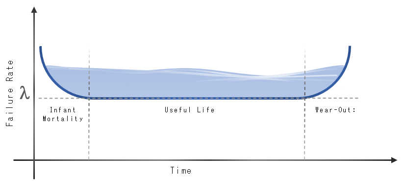
- early-life failures, where initial defects or commissioning issues may cause a higher failure rate;
- useful life, where the failure rate is relatively low and stable;
- wear-out, where aging, fatigue and degradation increase the probability of failure.
For engineering studies, the level of detail should match the objective of the analysis and the quality of the available data.
Reliability Block Diagrams
A Reliability Block Diagram, or RBD, represents the logical structure of a system. Each block represents an equipment item or subsystem, and the connections show whether the system depends on components in series, in parallel, or in a combination of both.
In a series configuration, all components must operate for the system to operate. If any component fails, the system fails.
In a parallel configuration, the system can continue operating as long as at least one path remains available. This is why redundant equipment can increase system reliability.
RBDs are useful because they provide a clear first representation of system logic. They help identify critical equipment, compare series and parallel arrangements, and estimate the reliability of simple subsystems.
Limitations of Static RBD Analysis in Mineral Processing
Although RBDs are valuable, mineral processing plants introduce additional complexity.
Material does not simply pass through a logical diagram. It accumulates in bins, stockpiles, tanks and sumps. Equipment can be starved, blocked, bypassed or operated at partial capacity. Control strategies may change flow rates, open or close routes, and prioritize one section of the plant over another.
These dynamic effects are difficult to represent in a purely static RBD.
A stockpile is a simple example. If upstream equipment fails, the downstream plant may continue operating while the stockpile is being reclaimed. If downstream equipment fails, the upstream plant may continue operating until the stockpile reaches its maximum capacity. The same equipment failure can therefore have different production consequences depending on stockpile level, reclaim rate, feed rate and operating logic.
This is why dynamic simulation can provide a more realistic reliability analysis for mineral processing circuits.
Reliability Studies with DPSIM
DPSIM combines reliability events with dynamic process simulation.
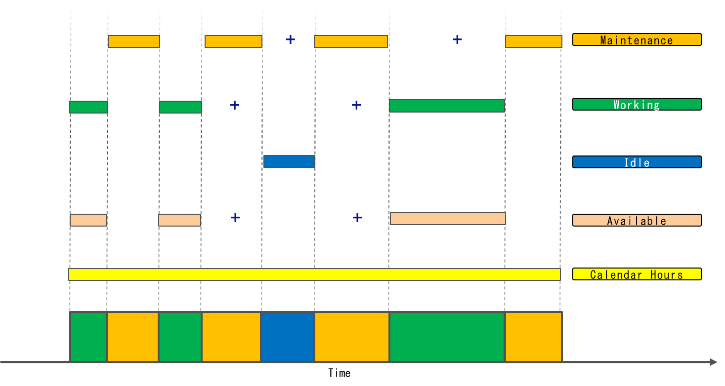
Instead of only calculating whether equipment is available or unavailable, DPSIM can simulate how failures and repairs affect the flowsheet over time. Equipment states, material flows, inventories, control rules and operating strategies can be evaluated together.
This allows engineers to investigate questions such as:
- How many operating hours can the plant achieve under a given reliability scenario?
- Which equipment failures have the greatest impact on production?
- How much buffer capacity is required to protect the downstream plant?
- Does a parallel route, bypass, standby equipment or operating rule improve production?
- Which bottlenecks appear only when failures and process dynamics are considered together?
By representing both the reliability behavior of equipment and the dynamic response of the process, DPSIM helps engineers move from component-level reliability indicators to plant-level production insight.