
What a separator predicts
A separator is a mapping from an incoming particle population to outgoing populations. The population carries size, composition and any other characteristic that the model resolves. A separation law specifies a fraction for each distinguishable class. The material balance then converts those fractions into tonnes, grades and recoveries. An optimized separator design, a fitted operation and an inverse calculation from product samples can all use the same bookkeeping while answering different questions.
The decisive question is which differences among particles the separation law can see. A size partition assigns the same probability to different components in one size interval. A component recovery transfers the same fraction of a component in every size interval. A size–density surface can distinguish a large light particle from a small dense particle. If the material representation does not carry density, liberation or susceptibility as a class variable, that information cannot appear in the calculated selectivity.
Distinguish a chemical assay from a material category. A particle containing 40% iron can include gangue and several iron-bearing minerals. A model entered with iron assay as though it were a magnetic volume fraction will act on a different quantity from the one measured. Bulk chemical grade is an output that can be synthesized from mineral composition through a grade matrix. Particle properties used for capture and sedimentation have to be defined separately.
Flow, yield, grade and recovery
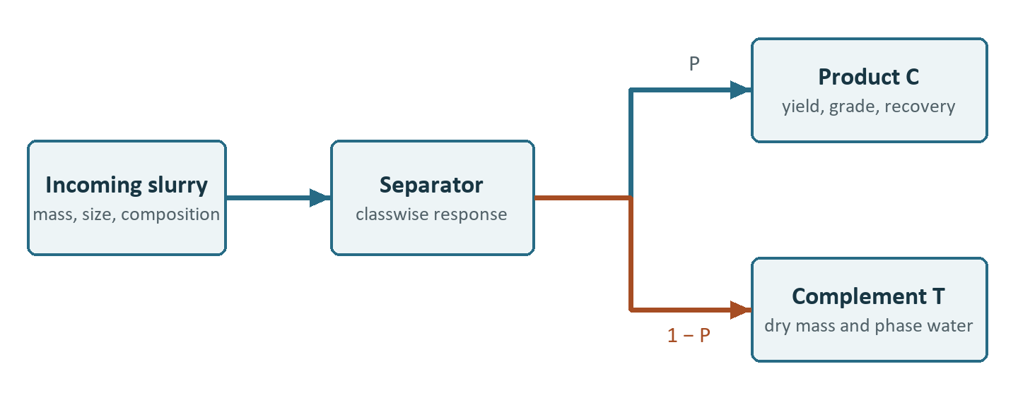
Let Fᶜᵢ be the dry feed flow of component c in size interval i, in t/h. A two-product separator assigns Pᶜᵢ in the closed interval [0, 1] to product C. The remaining fraction reports to product T.
Dry product flow is the sum over all the occupied classes. Dry mass yield Y is C/F. Product grade gᶜ is the mass of component c divided by the total dry flow in that product. Component recovery Rᶜ is the fraction of the feed mass of the component in the designated product. Denote bulk feed grade by fᶜ.
A zero denominator makes the associated grade or recovery undefined from the survey. A numerical placeholder in an empty product is not a measured zero. A balance review should retain flow and grade separately so a solver cannot hide a zero-flow condition behind an apparently accurate assay. Component and size recovery both require denominators at the same aggregation level. Averaging fractions without their feed mass weights generally gives a different result from averaging flow.
Water recovery should be tracked independently when the model gives water its own partition. If W is feed water flow in t/h and β is recovery to C, W꜀ = βW and Wₜ = (1 − β)W. This operation changes product slurry density and flow independently of its effect on solids. In flotation, water transfer can also enter the solids partition through entrainment. That coupling arises in the recovery law, while the phase balances remain separate.
Worked example 1. Resolving a misleading concentrate grade
Feed 120 t/h dry solids and 80 t/h water to a separator. Use two size intervals and two components, valuable V and gangue G. The feed has 30 t/h valuable mineral. Compare the response when the valuable material is liberated enough for the following class partitions to apply.
| Class | Feed solids (t/h) | Partition to C | C solids (t/h) | T solids (t/h) |
|---|---|---|---|---|
| Coarse V | 18 | 0.90 | 16.2 | 1.8 |
| Fine V | 12 | 0.65 | 7.8 | 4.2 |
| Coarse G | 42 | 0.10 | 4.2 | 37.8 |
| Fine G | 48 | 0.15 | 7.2 | 40.8 |
| Total | 120 | — | 35.4 | 84.6 |
The concentrate grade is 24/35.4 = 67.80% and the tailings grade is 6/84.6 = 7.09%. The valuable mineral recovery is 24/30 = 80%. The mass yield is 35.4/120 = 29.50%. Their identity check is 0.295 × 0.6780/0.25 ≈ 0.800. The concentration ratio F/C is 3.39, whereas the enrichment ratio gᵥ/fᵥ is 2.71. These ratios answer different questions.
For water recovery of 25%, the concentrate takes 20 t/h water and is 35.4/(35.4 + 20) = 63.90% solids by mass. The remaining product takes 60 t/h water. If the target concentrate is limited to 50% solids downstream, a separate dilution step requires 15.4 t/h water at this operating point. The added water alone leaves the dry grade and dry yield unchanged.
The bulk partition in the fine interval is (7.8 + 7.2)/(12 + 48) = 25%. That number says little about the fine valuable recovery of 65%. Two plant surveys with identical component-wise partitions can have different bulk partitions after the feed composition changes. To distinguish a genuine loss in capture from a change in feed mineralogy, compare matched classes or reweight the old partitions using the new feed.
Model forms and identifiability
A fixed per-component recovery model can represent a previously measured stage without inventing additional degrees of freedom. If independent observations show that coarse and fine grades respond differently, a size or size–component model can be appropriate. In the DPSIM family of separator models, component recoveries, component-dependent size curves, size partition and grade-targeted inverse models exist as distinct devices. User-specified recoveries are direct transfer fractions. A grade-targeted inverse model, such as Product Assay Separation, derives feasible transfer fractions from measured or specified product assays and can reconcile inconsistent inputs. Neither calculation makes a new mineral property appear in the feed description.
One simple size partition used by the Gravity Partition Separator rises with class diameter d. It interpolates between a low-size bypass B and high-size recovery M. With a cut-scale d₅₀ and sharpness n, define a dimensionless response U.
At d₅₀, the actual recovery is (B + M)/2. It equals 50% only when B + M = 1. A high M and a sizeable B can deliver a 70% actual partition at a nominal corrected cut of 50%. Use the model's named parameters to distinguish size cut, density cut and permeability-like characteristic values. Different models use superficially similar names.
When fitting size partitions, include measurements on both sides of the transition and in any plateau that is to be estimated. Data tightly clustered about the midpoint can constrain slope locally while leaving both plateaus poorly determined. With target grades or recoveries by component, test whether the measured feed actually contains enough of each component to produce the targets. A negative reconstructed flow or an apparent recovery above unity points to inconsistent observations, incompatible sample bases or a wrong process boundary.
Worked example 2. Inverse grade–yield calculation
For a steady two-product stage with feed value grade f = 0.25, concentrate grade c = 0.70 and tails grade t = 0.08, the mass balance gives f = Yc + (1 − Y)t. Solving for Y gives 0.17/0.62 = 0.27419, and value recovery is 0.27419 × 0.70/0.25 = 76.77%. Given 120 t/h feed this corresponds to 32.903 t/h concentrate, 87.097 t/h tailings and 23.032 t/h recovered value. Calculating the other outlet gives 87.097 × 0.08 = 6.968 t/h, taking the balance back to the incoming 30 t/h value.
This calculation becomes ill-conditioned when the two product assays are close. It can be impossible when f lies outside the interval spanned by c and t. Increasing the weight on one assay through reconciliation changes which observations the model honors most closely. It cannot cure an impossible sample definition. Inspect residuals in percentage points and compare them with sampling and analytical uncertainty.
Exercises and answers
- A plant reports 30% dry yield and 50% concentrate grade at 20% feed grade. Find valuable recovery and tailings grade. Answer. Recovery is 0.30 × 0.50/0.20 = 75%. Tailings grade is (0.20 − 0.30 × 0.50)/0.70 = 7.143%.
- A solids partition has B = 0.10, M = 0.90 and n = 2. Find the actual fractions at half and twice the cut scale. Answer. The underlying curves give 0.20 and 0.80, hence P = 0.26 and 0.74.
- Check a survey with f = 0.12, c = 0.10 and t = 0.04. Answer. The inverse yield is 1.333, so that set of assays cannot close a two-product balance. Check stream identification, coincident sampling and analytical bases before changing the separation model.
Reading
Wills and Finch, Wills’ Mineral Processing Technology, 8th ed. (2015), provides background on grade, recovery, size separation and process accounting. The active size partition and inverse examples are grounded in the DPSIM Gravity Partition Separator and Product Assay Separation implementations. Their numerical examples above use original data.