
What a flotation rate measures
In a well-defined bench test, suppose the mass M of a selected class remaining in the pulp loses a constant fraction in each short time interval. Under this assumption, dM/dt = −kM. The numerical value of k depends on the time unit. The rate 0.3 min⁻¹ is 0.005 s⁻¹ and 18 h⁻¹. The product kτ is dimensionless. For initially floatable mass, integration of the loss law gives the fraction recovered by elapsed time τ.
The derivative at zero is k, and the time to collect half of the population is ln(2)/k. Let F∞ denote the floatable fraction. True recovery to the froth on a feed mass basis is F∞ Rₖ. At short times this is approximately F∞ kτ, so early data alone estimate the product F∞ k. Long-duration data reveal a plateau, provided that reagent conditions and suspension remain sufficiently stable to preserve the model assumptions. Water-driven recovery of the remaining fraction can move the measured plateau away from F∞.
The same first-order survival law can be used for a particle with a known time in a collection zone. The continuous-flow question also requires a residence-time distribution. An ideally mixed cell has exit-age density exp(−t/τ)/τ, where τ = V/Q. Averaging particle survival exp(−kt) over that density gives 1/(1+kτ). Thus a batch test evaluated at the mean cell residence time predicts more recovery than an ideal mixed cell with the same k and τ. For N equal-volume ideal mixed cells of unchanged hydraulic flow in series, each cell has residence time τ/N and the unrecovered fractions multiply.
At kτ = 2, a single ideal mixed cell gives 66.67%, four stages give 80.25% and the exponential gives 86.47%. These comparisons apply at fixed total effective volume and unchanged flow. Water removal, changing component composition, reagent addition and aeration changes can alter the response of individual stages of a bank.
Rate distributions and size dependence
Uniform continuous distribution
A distributed-rate model starts with a population whose floatable particles have different values of k. In the active Distributed-Rate Flotation model, these values are uniformly distributed between kₐ and kᵦ. At a given elapsed time, integrate the remaining fraction across all possible rates and divide by the width of the range.
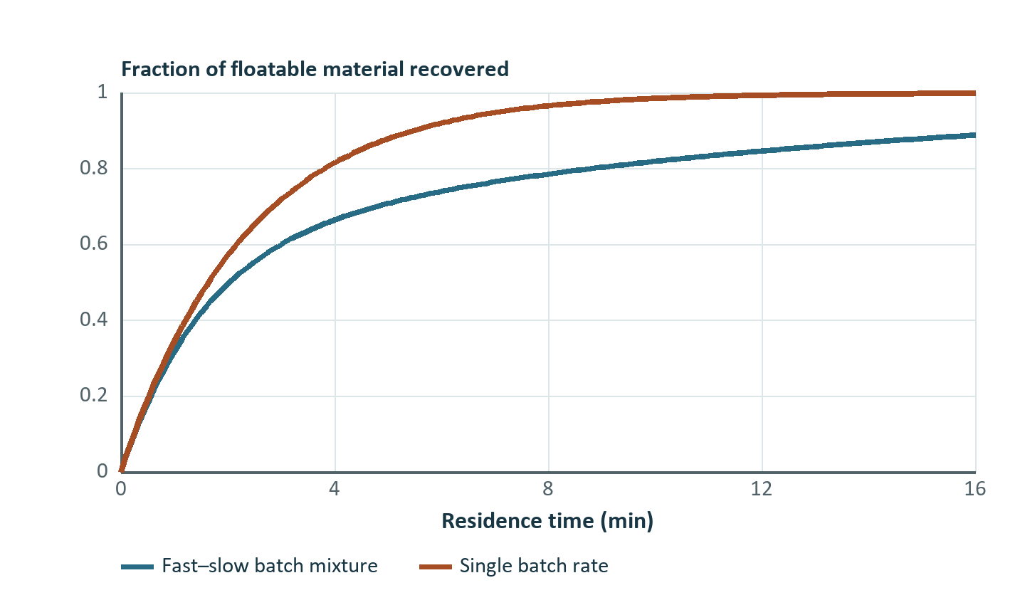
With identical endpoints the distribution collapses to a single rate and the exponential recovery is recovered as the limit. At positive τ the exponential survival is convex in k. Consequently, using the arithmetic mean rate in a single exponential overpredicts collection for a dispersed rate population. As time progresses, the fastest particles are preferentially exhausted, and the remaining mass is increasingly composed of slow particles. A decelerating apparent rate can therefore arise at constant reagent and aeration conditions.
This distribution describes heterogeneity in the batch kinetic rate. A residence-time distribution describes hydraulic heterogeneity. A measured recovery curve can reflect both effects. Fast and slow rates derived from a bench test do not identify the residence-time distribution of a plant bank.
Two rate groups
The active Fast-Slow Kinetic Flotation model uses two discrete groups with rates kfast and kslow, with p denoting the fraction of the floatable population assigned to the fast group.
The asymptotic true recovery is F∞ if both rates are positive. A zero-rate group and a lower floatable fraction can describe the same long-time behavior. Use the fewest free parameters supported by the time and mass resolution. Enforcing kfast ≥ kslow fixes the group naming. Even with that convention, rate pairs become weakly identifiable when the two estimated rates are close or one group is negligible. A model with two kinetic groups does not by itself identify two minerals or two liberation states.
Monotonic size-kinetic law
The Monotonic Size-Kinetic Flotation model applies the following size factor to each component's maximum rate kₘ, using representative size d, reference size dᵣ and sharpness n. The mineral-specific recovery follows the exponential at k(d) times the maximum floatable fraction.
At d = dᵣ, f = 0.5. The recovery at this size depends on τ, kₘ and F∞ and need not be 50%. Large d drives the rate toward kₘ. Use this law over ranges with an increasing size response. Broad feed ranges with slow ultrafines, a faster intermediate band and a coarse drop-off call for another response or evidence-supported subdivision. The water recovery input of this variant controls the water balance independently.
Entrainment and mass allocation
The active first-order, uniform-distribution and fast-slow variants combine kinetics with an empirical entrainment factor E. With feed-water recovery W, let B = clip(EW, 0, 1). Material already collected by true flotation leaves the remaining entrainment pool.
Here F∞ limits the true-flotation contribution. The simulated total can exceed F∞ when B is positive. These three variants use a common water-based factor across all component–size classes. It is a coarse proxy if the entrainment of gangue depends strongly on particle size or density. The circuit converts each class recovery to a mass rate and computes the tailings by subtraction. Actual solids concentration in the concentrate comes from its dry solids and water flows.
A size-dependent mechanical bank
In the active King Flotation Cell, the rate first multiplies an inverse square-root term, a coarse cutoff and an exponential penalty at fine sizes. With all sizes on the same configured micrometre basis and A fitted on that basis, the source implements the following for positive d.
Here dopt is a size-shape parameter. The rate peak depends on all terms, so infer it from the curve if required. Effective liquid–solid pulp volume divided by each cell feed flow sets τ in hours when V is in m³ and Q is in m³/h. Rates are numerically on a compatible hourly basis. The model evaluates total volumetric flow using class-weighted solid volume and available water. The recovered fraction per cell is kτ/(1+kτ). Solids to each next cell are the residual solids after that stage. It also computes internal water removal from the configured apparent froth solids fraction, bounded by available water. Check the final reported water and port direction for the selected water-routing setting when calibrating a bank. The physical destinations are Floated and Bottom, which anchor the assay accounting in either direct or reverse flotation. Treat the formula here as the active King-style compatibility model and fit A to measured class performance.
A single cell receives 40 m³/h of pulp. Its 16 m³ volume is 85% effective. Use d = 60 µm, dmax = 250 µm, dopt = 35 µm and A = 30 on the model's micrometre/hour basis.
If the incoming class mass is 10 t/h, 5.163 t/h floats from the cell. For a second cell, first recompute Q from remaining water and solids. Recalculating flow is particularly important in a low-flow cleaner with high mass pull. Raising the number of parallel banks at unchanged total flow and volume per cell increases total installed volume and lowers each bank's inlet flow. It differs hydraulically from adding a stage in series.
Worked comparison at a common elapsed time
At τ = 5 min, consider a uniform rate range of 0.1–0.9 min⁻¹ and a two-rate alternative with the same endpoints and a fast share of 0.4. The uniform distribution gives 0.85114 = 1 − (e⁻⁰·⁵ − e⁻⁴·⁵)/4. The two-rate distribution gives 0.63164 = 0.4(1−e⁻⁴·⁵) + 0.6(1−e⁻⁰·⁵). A single rate equal to the uniform distribution's mean, 0.5 min⁻¹, gives 0.91792. The two-rate case also has a different mean rate, 0.42 min⁻¹, so its difference combines changes in the first moment and the distribution's shape.
Now give the uniform case feed solids of 80 t/h at 30% valuable component by mass. Use F∞ = 0.90 for the valuable component and a true recovery of 0.04 for gangue. Water recovery is 0.25 and E = 0.60. The entrainment fraction of each residual component is 0.15.
| Feed class | Feed solids (t/h) | True recovery | Total recovery | Concentrate solids (t/h) |
|---|---|---|---|---|
| Valuable | 24.0000 | 0.76603 | 0.80113 | 19.2270 |
| Gangue | 56.0000 | 0.04000 | 0.18400 | 10.3040 |
| Total | 80.0000 | 29.5310 |
The concentrate grade is 65.108%. Of the 10.304 t/h gangue in concentrate, 2.240 t/h is assigned to true flotation and 8.064 t/h to entrainment. For water feed of 120 t/h, concentrate and tail water are 30 and 90 t/h. The concentrate is 49.60% solids by mass. The tail solids are 50.469 t/h and contain 4.773 t/h valuable component. Model selection changes both the grade calculation and the water duty downstream.
Calibration and exercises
Collect timed concentrates and assays, by size wherever possible. Plot incremental and cumulative recovery alongside water recovery. Measure solids mass independently of assay. Use early increments to constrain fast recovery and late increments for slow recovery or the floatable fraction. Fit the same combined response across runs with different water recovery to test how well it separates the two mechanisms. A single endpoint leaves kinetic rates, floatable fraction and entrainment strongly confounded. Keep a test condition, preferably a different size distribution or operating target, outside the fit.
- A class has F∞ = 0.8 and k = 0.25 min⁻¹. Compute true recovery at 4 min for a batch or plug-flow idealization and a well-mixed cell.
- In the two-rate law, kfast = kslow = k. Prove that the simulated kinetic curve is independent of p.
- Under the entrainment proxy, a component has a true recovery of 0.25 and total recovery of 0.40 at W = 0.20. Find E, assuming no clipping. Explain why the fit remains uncertain.
- In the numeric King case, compute the collected mass if one uses gross volume instead of effective volume with the same Q and k.
Answers
- Exponential true recovery is 0.8(1−e⁻¹) = 0.5057. The mixed-cell value is 0.8 × 1/2 = 0.4000.
- Factoring the common exponential recovery leaves p + (1−p) = 1.
- B = (0.40−0.25)/(1−0.25) = 0.20, giving E = 1. If the inferred 0.25 true recovery changes, E changes even with identical measured total recovery. Independent water or kinetic contrasts constrain the decomposition.
- τ becomes 0.400 h, R = 0.5567, giving 5.567 t/h for 10 t/h feed. The extra 0.404 t/h is driven by the residence-time assumption.
The active formulas are traceable to the DPSIM classes FlotationRecoveryCalculations, FlotationKineticEquipmentBase, their four kinetic variants, and FlotationKing. Wills and Finch (2016) provide flotation mechanism and equipment context.