
Size classes as material inventories
A continuous mill combines particle breakage with residence time. A material can leave coarse because its breakage rate is low, because the slurry leaves quickly, or because a breakage event produces mostly same-size daughters. The measured product cannot generally distinguish these mechanisms by itself. A population balance makes the ambiguities explicit by representing them as separate terms.
Consider one solid component and n size intervals from coarsest to finest. For interval i let Fᵢ be connected feed rate in t/h, Mᵢ its solids inventory in t, Rᵢ its first-order breakage rate in 1/h, Dᵢ its first-order discharge rate in 1/h, and bᵢⱼ the fraction of a breakage event from parent j that appears in interval i. Appearance columns describe mass fractions including same-size material. Breakage creates smaller particles with the same component identity. If a model represents particle composites as classes, liberation requires a richer state or a calibrated remapping. An ordinary PSD balance cannot infer liberation from mass conservation alone.
At steady state the left side is zero. Resolve the same-size appearance term into the loss coefficient to cancel its share of the breakage departure.
Since daughter mass moves to finer intervals, the balance is triangular. Solve the coarsest class first, pass its daughters to finer classes, and continue to the pan. A class must have a finite exit route if Uᵢ is positive. For example, an interval can have Dᵢ = 0 in a grate-controlled mill, but then Rᵢ(1 − bᵢᵢ) must be positive if connected feed or breakage daughters reach it. Refusing an impossible steady state is more informative than adjusting an inventory to an arbitrary large value.
A dry mass closure check follows by summing the differential equation across all classes. If every appearance column sums to one, breakage departures and daughter arrivals cancel over the full distribution. Then total feed equals total discharge at steady state. Closure should hold for each component. A negative retained fraction or a pan entry that disappears usually indicates an invalid appearance column, a class alignment mistake or an inconsistent discretization.
In the Calibrated Perfect-Mixing Mill (R/D), substitution of RᵢMᵢ = (Rᵢ/Dᵢ)Pᵢ into the preceding equations eliminates inventory. With rᵢ = Rᵢ/Dᵢ, solve Pᵢ = Uᵢ/[1+rᵢ(1−bᵢᵢ)] while accumulating bᵢⱼ rⱼ Pⱼ from coarser classes. The fitted ratio is dimensionless. The Calibrated Perfect-Mixing Mill (RiDi, steady state) instead retains the absolute Rᵢ and Dᵢ and calculates the inventory for each class. Both variants use conservative appearance distributions on the selected size mesh.
Residence-time interpretations
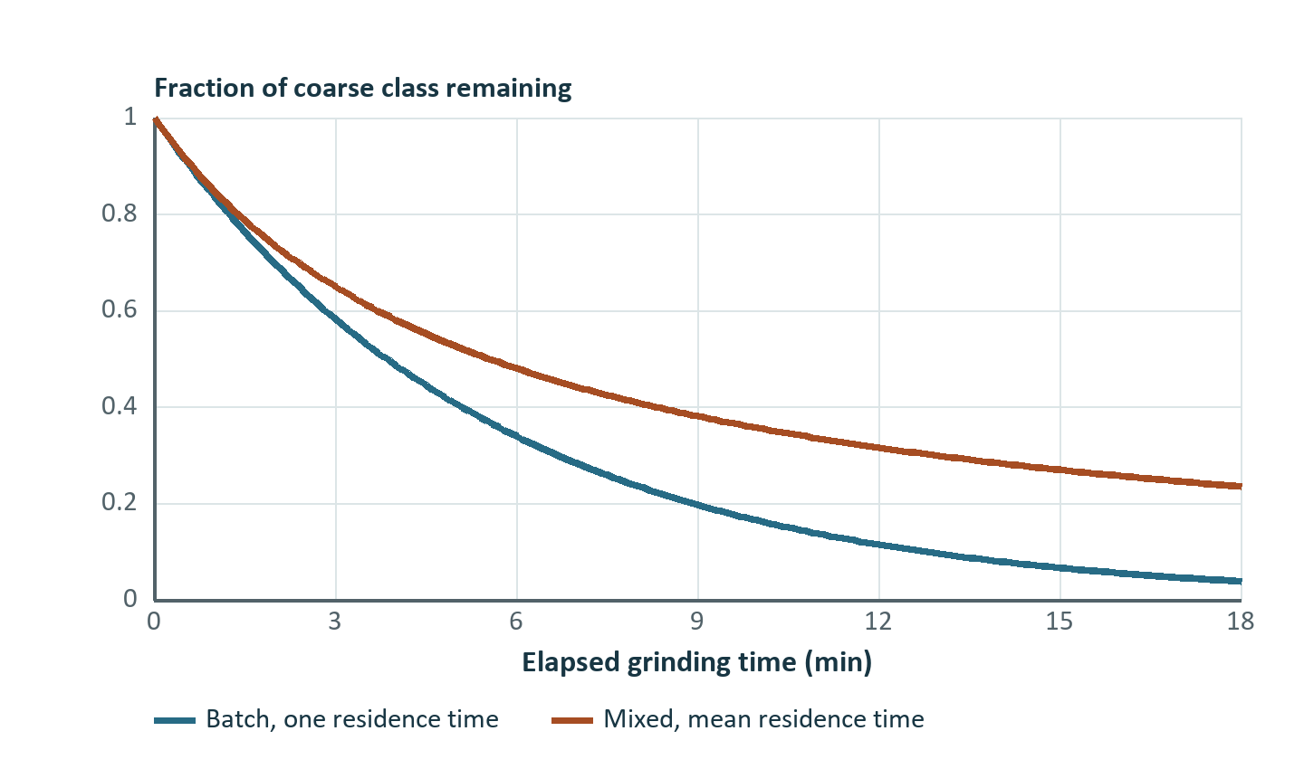
The single perfect mixer assumes that each particle has the same chance of leaving per unit time within a class. When discharge is size-independent, D = 1/τ and the liquid and solids share the same operating discharge rate by assumption. For a gross exposure τ divided among N identical perfect mixers, the residence time of each tank is τ/N. If one coarse class has a first-order disappearance constant k and its fine daughters never return to coarse, evaluate the coarse survival through N tanks from this expression.
The plug-flow limit as N increases is exp(−kτ). At equal mean residence time, a single perfectly mixed tank retains more coarse material in this example because the residence-time distribution has a larger short-residence fraction. Closed-circuit external recycle changes how many times a particle sees the mill and is still handled through the plant circuit. Internal tank count represents residence time within one pass.
Herbst–Fuerstenau grinding formulations scale the selection rate with net specific power delivered to a solids hold-up. A convenient convention is to define Sᴱᵢ in t/kWh and P/H in kW/t, with P net power and H solids hold-up. Then Sᵢ = Sᴱᵢ P/H gives a rate in h⁻¹, or divide by 60 for min⁻¹. Here P/H is power per tonne held in the mill. It is not plant specific energy P/Q. For a well-mixed steady vessel with H = Qτ, multiplying Sᵢ by τ yields Sᴱᵢ P/Q. This identity explains why some simplified balances can use energy per tonne of throughput directly and solve a series of energy steps without fitting a separate absolute residence time. It also shows why a product fit alone may leave the separate values of power, holdup and residence time indeterminate.
The general Herbst-Fuerstenau PBM Mill represents a specified specific-power and residence-time model. The Herbst-Fuerstenau Ball Mill derives operating quantities such as power, estimated hold-up and residence time from a ball-mill representation and applies its calibrated rate correction where selected. The two use the same energy-scaling idea with different closure of the machine duty. The reduced Population Balance Ball Mill, Population Balance Rod Mill and Population Balance Vertical Mill share a three-mixer form while using machine-specific calculations for energy, selection parameters or power. Their common numerical method does not imply equal breakage physics and setpoints across those machines.
Worked class-by-class inventory calculation
A two-class mill receives 100 t/h dry solids in the coarse interval and 80 t/h water. Let the coarse breakage rate be 3 h⁻¹, coarse discharge rate 2 h⁻¹ and fine discharge rate 1 h⁻¹. All coarse breakage forms the finer class. The fine class has no breakage transfer outside the tracked mesh.
The dry solids inventory is 80 t and discharge closes at 100 t/h. Feed water reports to product if the model has no withdrawal or addition. An R/D formulation yields the same PSD when the coarse ratio is 1.5 and appearance sends all coarse breakage to the fines. It needs the absolute discharge rates to recover the 80 t inventory. If both R and D at every size are doubled, the product remains 40 t/h coarse and 60 t/h fine, and hold-up falls to 40 t. This is an explicit parameter identifiability result.
At 100 t/h, a separate residence-time example with kτ = 1.5 gives 40 t/h coarse for one perfect mixer. With three equal stages the survival is (1 + 1.5/3)⁻³ = 0.2963, so 29.63 t/h coarse survives. Plug flow gives 22.31 t/h. These comparisons hold the same disappearance constant and mean exposure. Recalibrating k for each mixing assumption can reproduce a common measured PSD, which is why tracer data or measured inventory improve the model beyond a PSD fit.
Parameter estimation and use
Estimate appearance from restricted-size tests where feasible. Normalize daughter fractions on a consistent mass basis and include the same-size class. A cumulative breakage curve must be differenced carefully along descending apertures so retained fractions are positive. Then fit R/D to a survey while checking that residuals on fine and coarse samples don't reflect a classifier measurement bias. Introduce absolute rate scales only with inventory, transport or residence information. A curvature penalty or low-parameter selection law can help when there are many more size intervals than informative observations. Record the selected regularization as an assumption, not as independent process evidence.
A useful diagnostic is what happens when a model is moved to a different size mesh. One rate per interval calibrated on the old mesh generally cannot be copied by row number. Resampling a dimensional rate law and recomputing each appearance column respects the new apertures. The new result may still change because discretizing wide intervals changes represented mean sizes. Confirm converged trends by refining the mesh within the measured range, and guard the pan closure.
Exercises and solutions
- A class has R = 4 h⁻¹, D = 1 h⁻¹ and same-size appearance 0.6. It receives 26 t/h from feed and coarser classes. Compute inventory, direct discharge and daughter flow.
- In the worked two-class case increase the coarse discharge rate to 3 h⁻¹ without changing its breakage rate. Find the product split and total inventory.
- For kτ = 2, compare coarse survival with one and four tanks in series.
Solutions. (1) Net removal rate is 1 + 4 × 0.4 = 2.6 h⁻¹, so inventory is 10 t, direct discharge 10 t/h and daughter flow 16 t/h. (2) Coarse inventory is 100/6 = 16.667 t, with 50 t/h direct product and 50 t/h daughter flow. Fine inventory is 50 t, so total is 66.667 t. (3) The fractions are 1/3 and (1 + 2/4)⁻⁴ = 0.1975. The difference comes from residence-time shape at the same mean exposure.
Selected references. Herbst and Fuerstenau (1980), population-balance grinding mill scale-up. Lynch (1977), mineral crushing and grinding circuits. Whiten (1974), autogenous mill population balances.