
A particle size distribution is “measured” only after a measurement principle and a population basis have been specified. A test sieve classifies by the ability of differently shaped particles to pass apertures under a prescribed procedure. Optical or laser observations infer an equivalent size under physical assumptions about particle shape, scattering and dispersion. A set of image-derived particle counts weights the population differently from a dry mass sieve analysis. A thousand small grains may carry less mass than one coarse grain. Agreement of medians between these methods can occur by chance and gives little assurance about the tails.
The cumulative passing fraction F(d) is the fraction of dry solids mass in particles assigned a size no greater than d. It is nondecreasing, starts at zero in the ideal positive-size limit and tends to one. A differential size fraction is an integral over a finite interval, derived by subtracting adjacent cumulative values. A table of class mass fractions has a direct balance interpretation even when no smooth density exists within a class. A cumulative passing curve has an interpolation interpretation. This distinction matters whenever a model predicts x% passing a size that was missing from the sieve stack.
Sieve boundaries and interval masses
Suppose the apertures d₁ > d₂ > … > dₙ are ordered descending. The mass fraction above d₁ is 1 − F(d₁). The fraction in size interval (dⱼ₊₁, dⱼ] is F(dⱼ) − F(dⱼ₊₁). The pan fraction below the smallest sieve is F(dₙ). The differences telescope to one. The pan has an observed mass and no observed lower support. In the top class the total oversize sets a finite mass in an open-ended interval, with no measured maximum size.
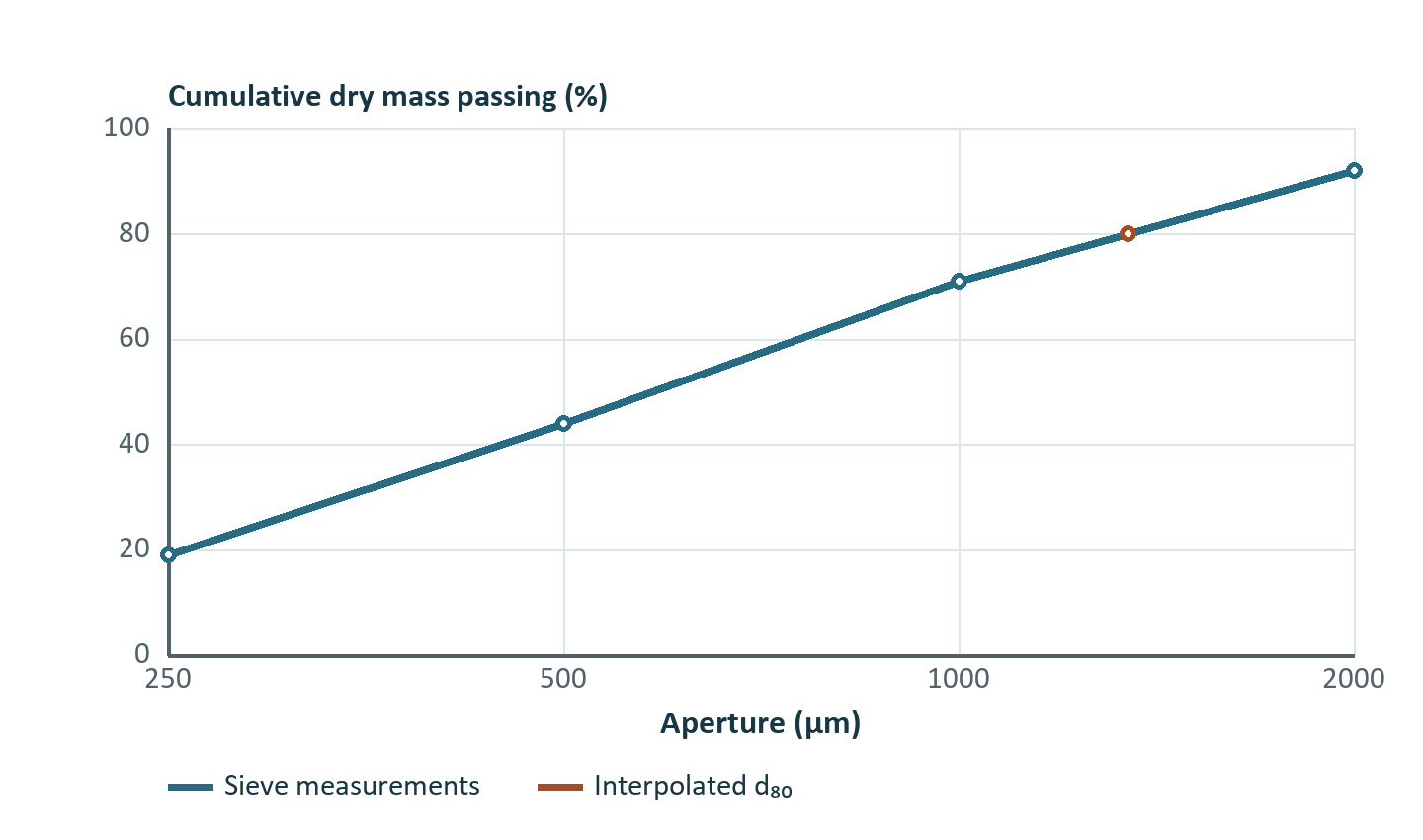
| Sieve aperture, µm | Measured mass retained, kg | Mass passing aperture, kg | Passing fraction |
|---|---|---|---|
| 2,000 | 0.80 | 9.20 | 0.92 |
| 1,000 | 2.10 | 7.10 | 0.71 |
| 500 | 2.70 | 4.40 | 0.44 |
| 250 | 2.50 | 1.90 | 0.19 |
| Pan | 1.90 | — | — |
The first retained mass corresponds to the open top class. The second is the fraction above 1,000 µm and at or below 2,000 µm. A model that evaluates the breakage rate in that bin at exactly 1,000 µm uses a boundary in place of a representative size. An interior value such as the geometric mean 1,414 µm can be suitable for logarithmically spaced classes, but a wide open-ended class needs an observed or independently specified top-size convention.
Moving a chart from micrometres to millimetres divides the displayed apertures by 1,000. The same classes, cumulative fractions and particle rates must survive the unit transformation. A predicted law t(d/d₅₀) should produce exactly the same fractions when every length is converted consistently. A law calibrated on d in µm with a dimensional coefficient requires that coefficient to transform as well. For example, the number used for a factor k in k d² changes by 10⁶ if the length variable changes from a numerical value in µm to one in mm and the same physical prediction is wanted.
Percentiles and interpolation assumptions
Let q fall between adjacent cumulative measurements Fₗ and Fᵤ at dₗ and dᵤ. In a piecewise linear model on log size, solve the interpolation directly. Natural or base-10 logarithms give the same answer if used consistently.
For the table above, the 80% passing size is between 1,000 and 2,000 µm. The interpolation parameter is (0.80 − 0.71)/(0.92 − 0.71) = 0.428571, giving about 1,346 µm. Linear d interpolation would give 1,429 µm. The difference is 6% despite exactly matching measurements. The midpoint in log size is standard for many plots containing a wide range of apertures, but the validity of the interpolation is controlled by the data spacing, measured curvature and chosen application.
An apparent d₈₀ can move across a measurement gap during calibration without a smooth change in individual class masses. This behavior matters when d₈₀ is the sole target. A candidate predicted curve can match d₈₀ while producing an incorrect amount of −250 µm dust and a radically different progressive transfer function. Add cumulative comparisons at multiple screens or compare actual class fluxes. If using all cumulative passing points in a least-squares fit, their residuals share information because neighbouring cumulatives contain many of the same size fractions. Diagonal weights then give a repeated vote to certain sample components. Better alternatives are comparing independent interval masses with a covariance model or selecting practical response points and acknowledging their dependence.
The pan and the open top deserve special consideration. If the smallest sieve passes 19%, d₁₀ is censored below 250 µm. It cannot be deduced from the table without an assumption on the missing tail. A fit can produce a numerical d₁₀, and different plausible tails can disagree greatly. Report it as inferred from that fitted curve. If a separator depends strongly on material at 90 µm, an additional measurement around that point is more persuasive than a simulated fine tail.
Grid changes and conservation
When merging neighbouring measured classes, sum their masses and component masses. No interpolation is needed. Refining a class is an inference. A conservative log-uniform rebin partitions each original interval in proportion to the log length of its overlaps with new intervals. Let interval (a,b] and target interval (u,v] have positive bounded endpoints. Allocate zero if they do not overlap. Otherwise allocate the fraction below.
Each source interval must allocate all its mass across the target grid, including open classes. Rebinning each constituent with the same source-bin weights conserves constituent masses. It assumes composition is uniform within the source class. If constituent distributions are independently measured, use those distributions and re-derive bulk solids classes from the constituent masses instead of interpolating bulk and component grades separately.
The example below shows 6.0 t/h in the 125–500 µm class with 0.60 t/h tracer. Insert boundaries at 250 and 350 µm. The log widths relative to ln(4) are 0.5000, approximately 0.2427 and 0.2573. The resulting predicted mass flows are about 3.00, 1.46 and 1.54 t/h. Each inferred class remains 10% tracer. These correlated estimates share a single observation. Counting them as three independent measurements in calibration invents precision.
Comparison near an operating cut
Consider an underflow partition that changes from 0.20 at 100 µm to 0.85 at 400 µm. A broad size bin with 20 t/h spans the entire transition. Three model choices give meaningful bounds. If all material is near 100 µm, the predicted underflow contribution is 4 t/h. If all is near 400 µm, it is 17 t/h. Using the geometric midpoint 200 µm with a log-linear partition gives 10.5 t/h. An independent size measurement shows 80% of the class mass near 100 µm and 20% near 400 µm. The calibrated prediction over the broad bin is then 0.8 × 4 + 0.2 × 17 = 6.6 t/h. Refining the mesh in software is useful only if physical information or an explicit inference supports the refinement.
For integration over an arbitrary representative density f(d), the effective class partition is the mass-weighted mean, ∫t(d)f(d) dd / ∫f(d) dd over the bin. The representative diameter is an approximation to this weighted mean response. Convergence of the prediction as one refines the grid under an assumed density establishes numerical consistency with that density. It leaves the inferred density itself to be validated.
Measurement credibility
Retained fines can agglomerate during drying or sieve blinding. Particle breakage during preparation may shift the distribution in the opposite direction. For a wet screen feed with clay, classify the operational meaning of “fines.” A laboratory dispersed distribution can be the right variable for a mineralogical analysis and an overly optimistic proxy for plant sieving at a given water rate. Record the preparation method and inspect which measurement best reproduces the physical population relevant to the model. Repeat samples and compare the repeatability where it matters, such as the material just below a screen aperture.
A particle image counting analysis may be converted to a mass-like distribution only under explicit assumptions on particle volume and density. For equal-density spherical particles, weight each count by d³. For a mixture of densities, weight by ρd³ and account for shape factors or measurement bias. In a population containing one 1,000 µm particle and 1,000 particles of 100 µm, the coarse particle provides about half the mass under the equal-density spherical assumption. It is only about 0.1% of the count.
Exercises with solutions
Exercise 1. Estimate d₅₀ for the sieve results. Which observations make it identifiable?
The 500 and 1,000 µm sieves bracket 50% passing. The exponent is (0.50 − 0.44)/(0.71 − 0.44) = 0.22222. The estimate is 500 × 2^0.22222 ≈ 583 µm. If either reading were missing, wider bracketing might change the estimate. A slope using the whole range need not equal the local interpolation slope.
Exercise 2. A chart compares a calculated curve entered in µm with lab points entered in mm. Its calculated d₈₀ is 740 in file units, and the measured d₈₀ on its own chart is 0.735. Compute the relative size error.
The two d₈₀ values are 740 and 735 µm. The relative size error against measurement is approximately +0.68%. The numerical size difference, read without units, appears nearly three orders of magnitude too large.
Exercise 3. A 100 kg sieve run recovers 96 kg, with 12 kg in the pan. Compare the 12%, 12.5% and 16% fine fractions that can be quoted from these figures.
The measured pan mass is 12% of the initial sample and 12.5% of the recovered mass. The upper bound from an assumption that all missing mass would have entered the pan is 16% of initial mass. Representing the pan as exactly 12.5% assumes the recovered material is a suitable representation of the loss. Recovering retained fines from handling surfaces or repeating the test addresses the issue directly.