
Begin with one destination
A partition curve gives the fraction of the feed of a specified size recovered to a specified outlet. Let pᵢⱼ be the actual partition to the coarse outlet for size class i and component j. For feed solids Fᵢⱼ in t/h, the two product cells are
The same equation uses fine or overflow as the reference destination if every p is redefined as recovery to that outlet. Reversing a partition means replacing p with 1−p and changing the definition of the total recovery. An ideal sharp cut places all particles above the chosen size in one stream and all below in the other. An interval intersecting the cut is resolved with the designated within-class interpolation. Assigning the entire interval according to its midpoint can cause a discontinuous predicted response when an aperture changes slightly.
The total solids recovery to coarse is ΣCᵢⱼ/ΣFᵢⱼ. If one common curve is used for all components, a given component can still recover preferentially because its feed distribution is coarser. Conversely, a total partition computed from measurements can drift when the component proportions change even if the component-specific partitions are unchanged. A partition for a valuable component is its recovery from its own feed mass, with all accumulation and sampling bases defined consistently.
Deriving partitions from a survey
Let cᵢ and fᵢ be the mass fractions in class i of the coarse product and feed. If Rₛ is the total feed solids recovery to coarse, the measured recovery for that class is
With both product size distributions and a reconciled flow balance, an equivalent estimate is Rₛcᵢ/[Rₛcᵢ + (1−Rₛ)uᵢ]. Both require size distributions on the same sieve boundaries and solids basis. The equation divides by fᵢ, so an almost empty class can produce a very uncertain p even when the absolute mass error is small. A class with fᵢ = 0 provides no observation of pᵢ. A fitted curve may predict p there. Report that prediction with its basis.
A weighted fit can use residuals in recovered mass, predicted and measured product masses, or measured partition with uncertainty weights. Giving all percentages the same influence can fit a nearly empty class at the expense of a plant-critical class. Where the source is measured component assays, errors in element-to-mineral conversion and mineral liberation can propagate into component partitions. Test a total mass-by-size balance before fitting component-specific curves.
Water recovery and correction
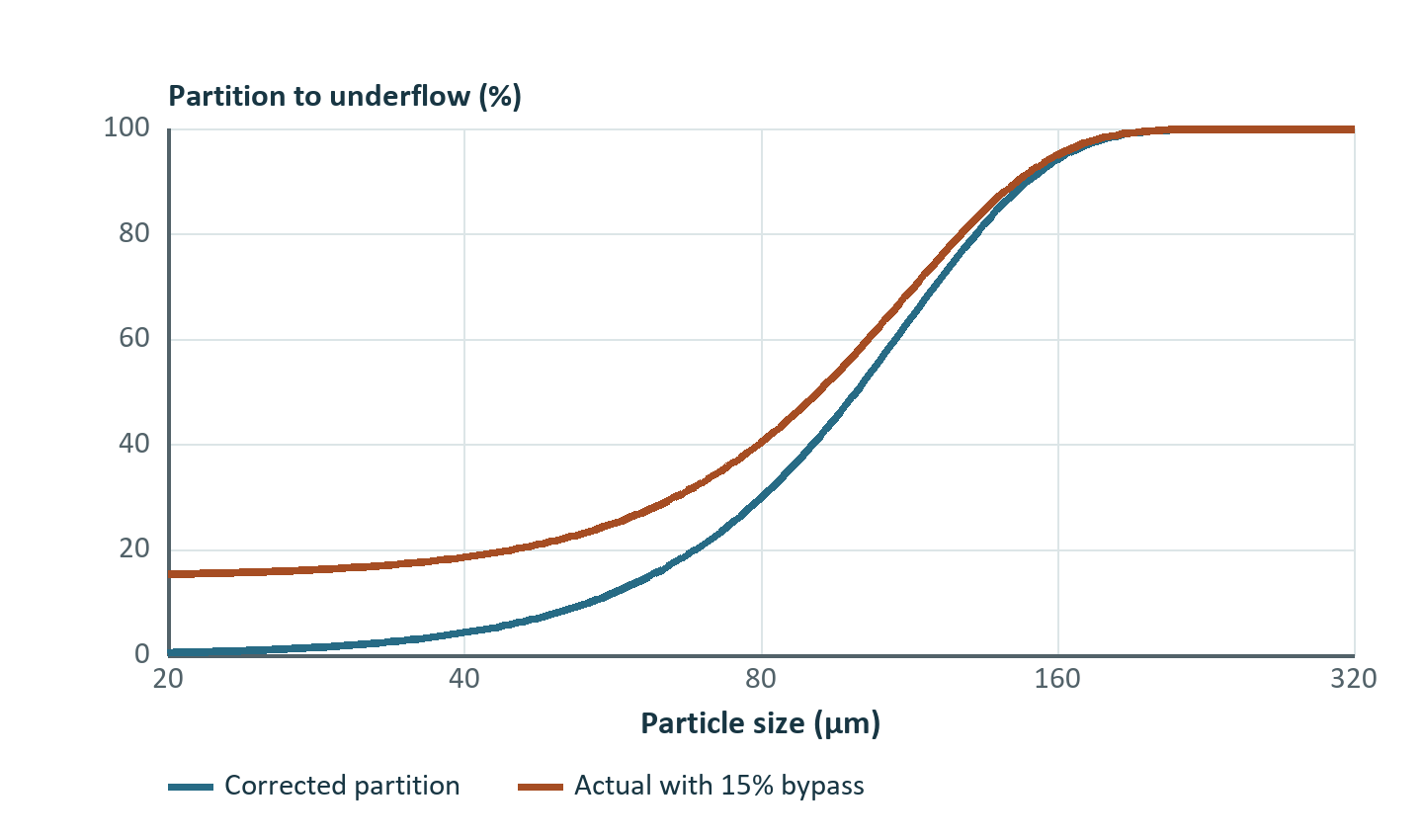
Let b = W꜀/W𝒻 be the fraction of feed water to the same coarse outlet. A common hydraulic idealization sends b of the particles with the water and subjects the remaining fraction to a size-selective coarse recovery Eᵢ.
The correction assumes water-entrained solids bypass contribute a size-independent floor at b. It applies when that approximation is suitable. Measured fine-class recovery below b signals a sampling inconsistency or behavior outside that approximation. Fitting a clipped corrected curve can suppress the very residual that diagnoses the problem. A measured water split alone cannot identify possible extra fine retention, fish-hook behavior or a coarse end that approaches less than complete recovery.
Choose the corrected law to suit the shape observed. A logistic form E(x) = 1/[1 + (d₅₀꜀/x)ᵅ] gives 50% corrected coarse recovery at x = d₅₀꜀. The Rosin–Rammler form E(x) = 1−exp[−ln(2)(x/d₅₀꜀)ᵅ] has the same midpoint but a different tail. The exponent α is specific to each law. Fits of α across different families are comparable only by evaluating a common curve metric or percentile width. Even with the same corrected law, the raw 50% coarse point changes with b.
An ordered spline uses measured size and partition knots to interpolate a curve with more freedom than a two-parameter sigmoid. Endpoint limits and interpolated values between knots deserve inspection. A bounded curve model prevents negative recovered masses. Monotonicity is useful when separation improves continuously with size, while a reproducible hook may justify additional shape freedom. A sparse survey rarely warrants many unconstrained knots. For a wide class, evaluate the influence of the class average partition and alternative within-class representations rather than relying on a single representative size.
Worked example with a component cross-check
The feed contains 30, 50 and 20 t/h in three size intervals from coarse to fine, and contains 60 t/h of water. Coarse outlet partitions are 0.98, 0.65 and 0.25. Water to the same outlet is 12 t/h.
| Quantity | Coarse interval | Middle interval | Fine interval | Total |
|---|---|---|---|---|
| Feed solids, t/h | 30.0 | 50.0 | 20.0 | 100.0 |
| Coarse product solids, t/h | 29.4 | 32.5 | 5.0 | 66.9 |
| Fine product solids, t/h | 0.6 | 17.5 | 15.0 | 33.1 |
| Corrected coarse partition | 0.9750 | 0.5625 | 0.0625 | 0.58625 |
Here b = 0.20. The corrected total is (0.669−0.20)/0.80 = 0.58625, or the feed-weighted mean of the three corrected class values. Coarse product is 66.9/(66.9+12) = 84.79% solids by mass. Fine product is 33.1/(33.1+48) = 40.81% solids by mass. With each component density 3.00 t/m³ and water density 1.00 t/m³, the coarse product contains 22.3 m³/h of solids and 12 m³/h of water, or 65.01% solids by volume. Mass and volume fractions answer different questions.
Suppose only 8 t/h total of a valuable component is present, with 1, 3 and 4 t/h across the three classes. Recovery of that component to coarse is (0.98+1.95+1.00)/8 = 49.13%, compared with 66.90% for all solids. The difference follows entirely from the distribution of the valuable component by size. A truly component-specific partition requires evidence that particles with different component compositions split differently even at comparable size.
Selection of a partition model
| Available evidence | Suitable first representation | Quantity to verify |
|---|---|---|
| Aperture or target cutoff, sparse sampling | Ideal size partition with a declared interpolation rule | Mass near the cutoff |
| Measured solids flow and several survey classes | Parameterized or spline partition | Partition of each class and integrated products |
| Component-specific size and product surveys | Partition per component | Component and solids balance simultaneously |
| Coarse outlet water split and a valid entrainment hypothesis | Corrected curve with a hydraulic term | Fine-class floor and water balance |
| Desired product percentile plus a parent curve shape | Inverse cut-size estimate | Target feasibility and predicted product yield |
This is a hierarchy of information requirements. A simple size cut can be appropriate in a preliminary balance even if a production deck behaves nonideally. Likewise a fitted spline can reproduce one survey precisely while extrapolating poorly when feed size or flow changes. The choice depends on the operating question and available evidence.
Exercises and solutions
1. Recovering partition from sizes
Coarse product is 60 t/h from 100 t/h feed. A class is 12% of feed solids and 18% of coarse product solids. Find its partition.
Solution. Recovered mass is 60 × 0.18 = 10.8 t/h. Feed class mass is 100 × 0.12 = 12 t/h. The coarse partition is 10.8/12 = 0.90.
2. Corrected midpoint
Water recovery to coarse is 0.25. What actual recovery corresponds to a corrected cut size?
Solution. p(d₅₀꜀) = 0.25 + 0.75 × 0.5 = 0.625. A point with actual recovery 0.50 instead has corrected recovery 0.3333.
3. Curve diagnosis
Near the fine end a measured p = 0.08, with water recovery to coarse of 0.18. What does the constant-bypass correction imply?
Solution. E = (0.08−0.18)/0.82 = −0.122. This is incompatible with the proposed floor. Reconcile the assays, flows and sampling first. If the difference is repeatable, test a different entrainment mechanism or curve form.