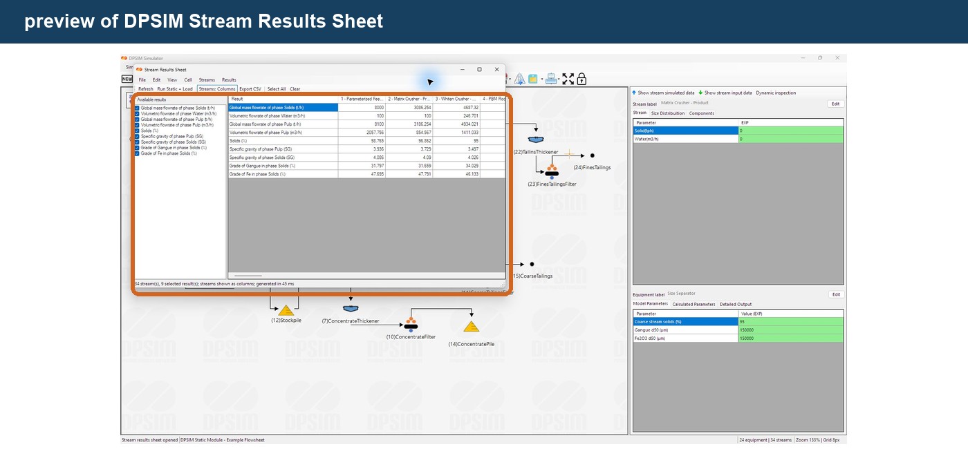
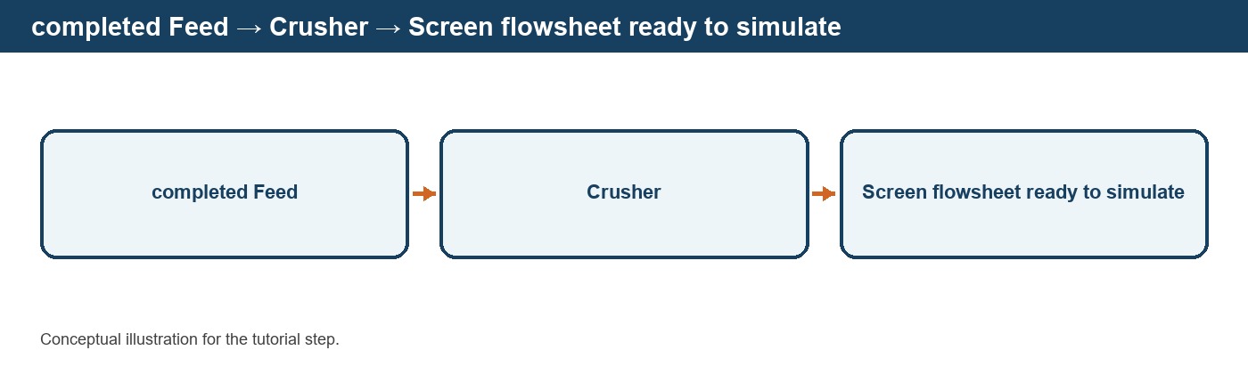
We now have everything required to perform our first calculation:
Material
The feed flowrate, water, particle size distribution and composition have been defined.
Flowsheet
The process units have been added and connected by material streams.
Models
The equipment parameters have been configured.
The next step is to run the simulation.
The DPSIM Static Module calculates the flowsheet under steady-state conditions, propagating the material through the selected process models and updating the resulting streams.
In this tutorial you will learn how to:
- run a static simulation;
- understand how DPSIM propagates material through the flowsheet;
- understand why the static solver uses iterations;
- recognize the effect of recycle streams;
- follow simulation progress;
- distinguish completion from convergence;
- perform basic checks after a simulation;
- troubleshoot common setup problems.
What does a static simulation calculate?
In a static simulation, we are interested in the condition of the process after the flowsheet has reached a consistent operating state.
Time is not explicitly advanced as part of the process calculation.
Instead, DPSIM determines the material conditions throughout the circuit based on:
feed conditions
flowsheet connectivity
equipment models
model parameters
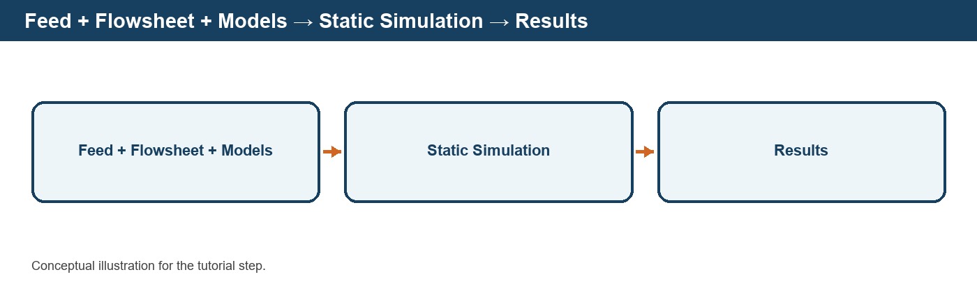
For every process unit, the mathematical model receives one or more input streams and calculates its output streams.
For example:
Feed → Crusher → Product
The crusher receives the feed particle population and calculates a new product particle size distribution.
That product may then become the input to another equipment model.
Conceptually:
Stream → Model → Stream → Model → Stream
This process continues throughout the flowsheet.
Running the simulation
To start the calculation, select:
Simulation → Run Static Simulation
or use the main simulation button on the toolbar.
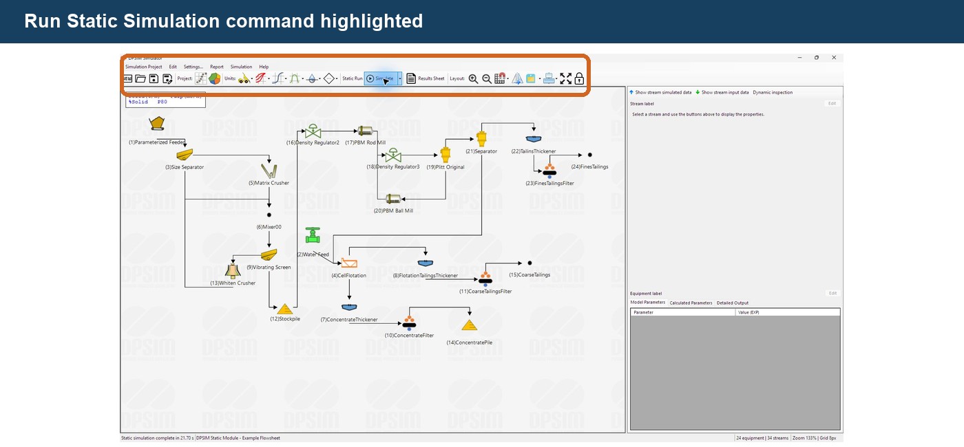
DPSIM starts processing the flowsheet.
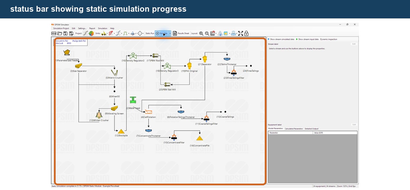
During the calculation, the status area displays the simulation progress.
For example:
Static simulation iteration 1 of …
When the calculation finishes successfully, the status changes to:
Static simulation complete
and may also display the elapsed calculation time.
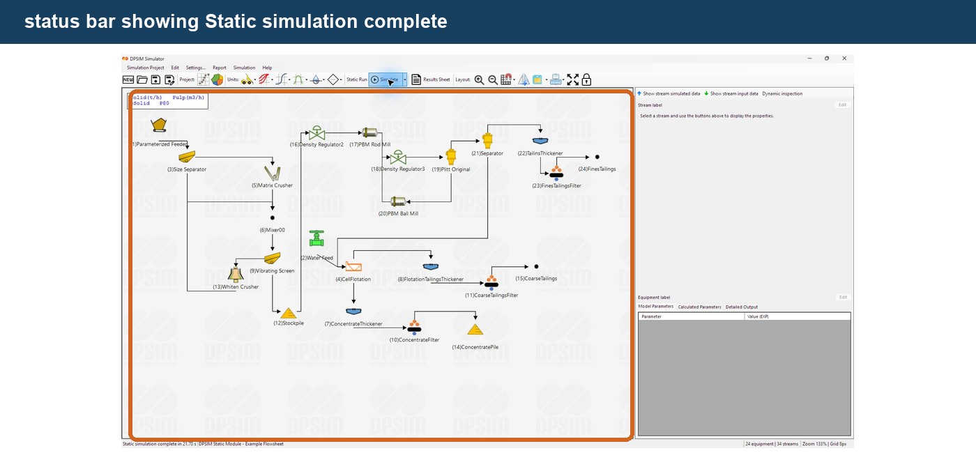
The stream and equipment results are then refreshed using the calculated values.
How material moves through the flowsheet
Consider the simple flowsheet developed throughout this series:
Editable Feed → Crusher → Screen
The feed stream already contains:
- solids flowrate;
- water flowrate;
- PSD;
- component composition.
The crusher receives this information.
Its model calculates the crusher product.
That product becomes the feed to the screen.
The screen model then calculates:
Oversize
and:
Undersize
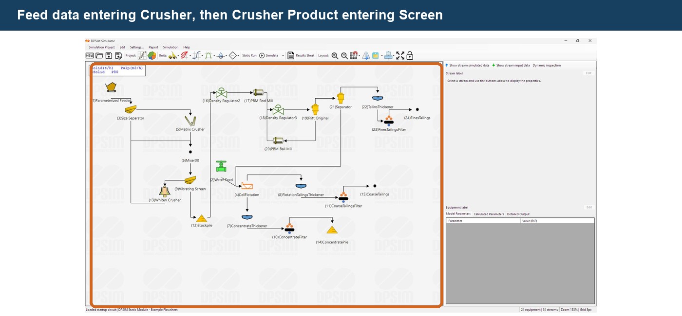
In this way, the material description created at the beginning of the project is progressively transformed by the process models.
The same principle applies regardless of the circuit size.
A complete plant is essentially a larger network of:
streams
and
unit-operation models
connected together.
Why does the static solver use iterations?
For a simple open circuit, the material can be propagated from the feed toward the final product relatively directly.
For example:
Feed → Crusher → Screen → Product
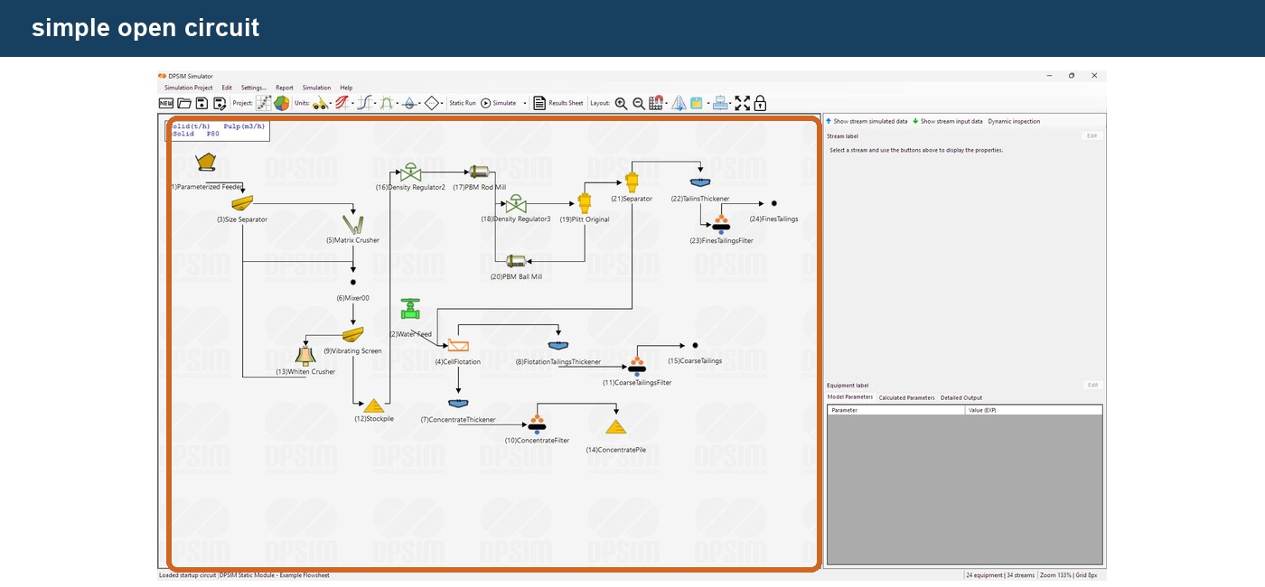
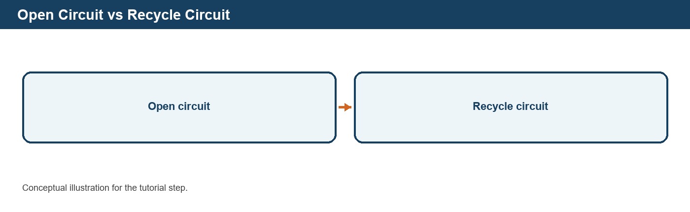
Now consider a closed circuit:
Mill → Cyclone
with:
Cyclone Underflow → Mill
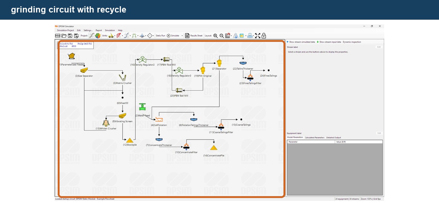
The mill feed depends on the cyclone underflow.
But the cyclone underflow depends on the mill product.
Therefore, the recycle stream cannot be determined independently in a single forward calculation.
The solution must be updated repeatedly.
Conceptually:
Initial estimate
↓
Calculate circuit
↓
Update recycle
↓
Calculate circuit again
↓
Update recycle again
↓
Continue until the results become stable
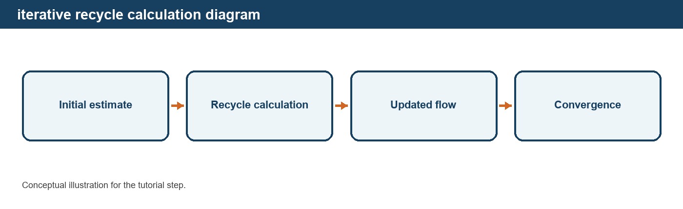
DPSIM therefore executes repeated static calculation passes through the flowsheet.
Understanding static iterations
Each iteration recalculates the process using the stream conditions currently available.
For a recycle circuit, the result of one pass becomes part of the input for the next pass.
Imagine the recycle flow evolving as:
Iteration 1 → 300 t/h
Iteration 2 → 430 t/h
Iteration 3 → 472 t/h
Iteration 4 → 486 t/h
Iteration 5 → 490 t/h
Iteration 6 → 491 t/h
The values are approaching a stable solution.
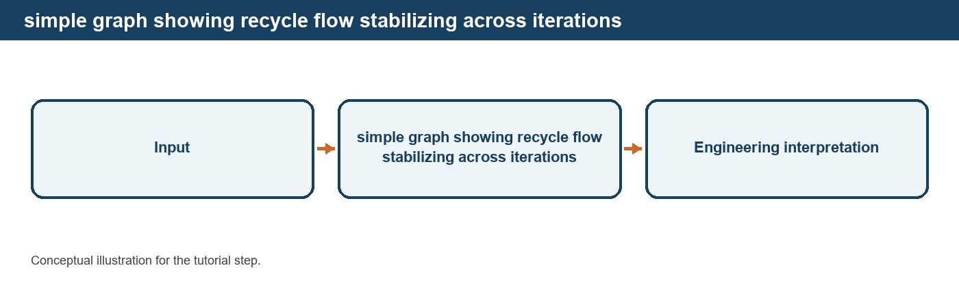
This is the basic idea behind iterative steady-state simulation.
The actual values depend entirely on the circuit and models being simulated.
Simulation completion and convergence are not the same thing
This distinction is important.
When DPSIM reports:
Static simulation complete
it means the configured simulation iterations have finished successfully.
It does not by itself prove that a recycle circuit has numerically converged.
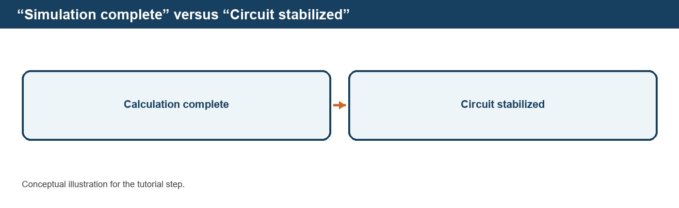
The current static solver performs the configured number of iterations.
Therefore, for circuits containing recycles, the user should verify that important stream values are no longer changing significantly with additional iterations.
For example, monitor quantities such as:
- recycle solids flowrate;
- circulating load;
- product flowrate;
- P80;
- component grade;
- percent solids.
Engineering note
A solver finishing without an error means the equations were executed.
Engineering convergence means that additional iterations no longer materially change the circuit solution.
These are different checks.
How many iterations are required?
There is no universal number that is appropriate for every flowsheet.
A simple open circuit may require very few calculation passes.
A closed circuit can require more iterations because information must travel repeatedly around the recycle loop.
The required number depends on factors such as:
- number of recycle loops;
- strength of the recycle;
- sensitivity of the equipment models;
- flowsheet topology;
- interactions between unit operations.
DPSIM allows the maximum number of static iterations to be configured.
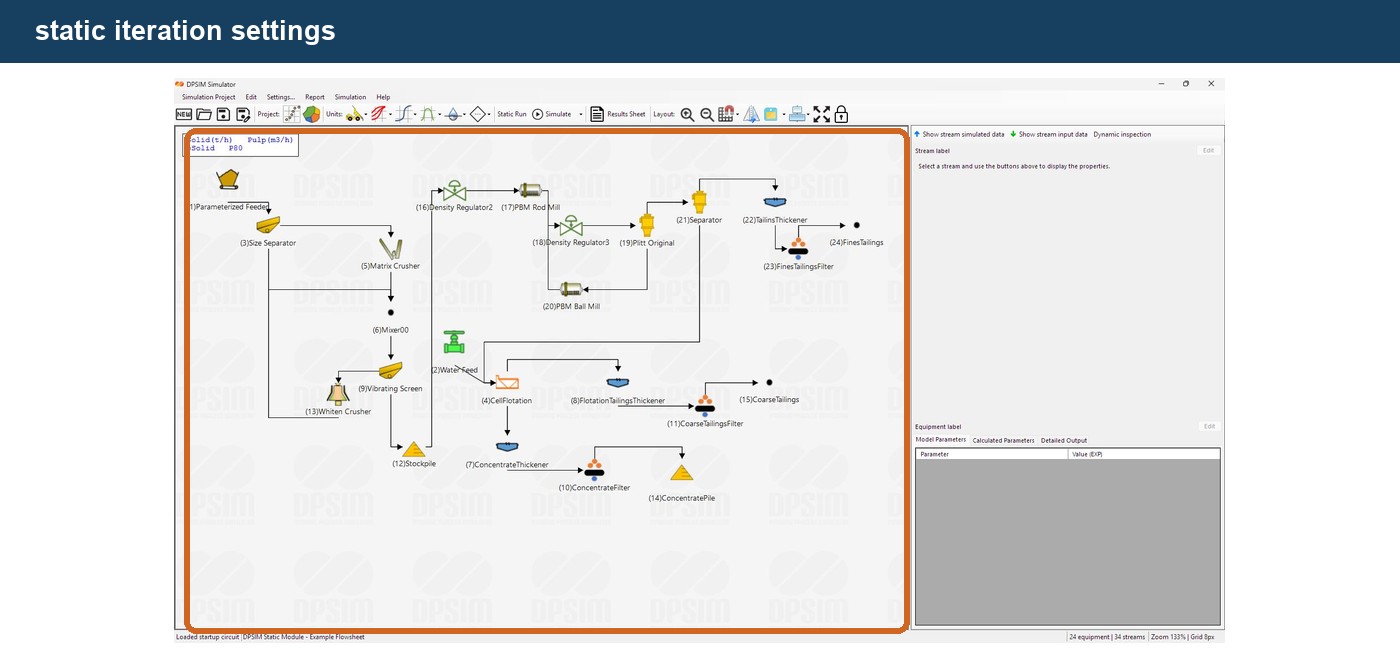
For a circuit with no recycles, increasing the iteration count excessively normally adds little value.
For recycle circuits, enough iterations should be used for the important calculated streams to stabilize.
A practical convergence check
A simple way to test a recycle circuit is to run the simulation and record one important recycle variable.
For example:
Cyclone Underflow Solids = 485 t/h
Run additional iterations.
If the result becomes:
486 t/h
and later:
486 t/h
the circuit appears stable for that variable.
If instead it changes to:
530 t/h
the solution is clearly still evolving.
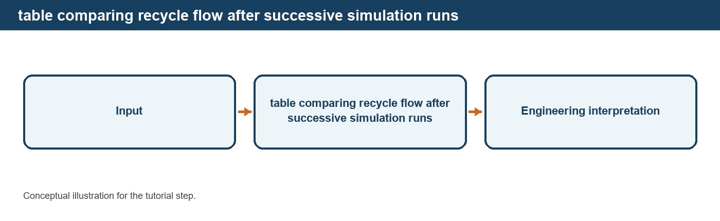
A stronger check is to inspect several important variables rather than only one.
For a grinding circuit, for example:
| Variable | Previous | Current |
|---|---|---|
| Cyclone underflow solids | 486 t/h | 486 t/h |
| Mill feed solids | 686 t/h | 686 t/h |
| Cyclone overflow P80 | 148 µm | 148 µm |
| Circulating load | 243% | 243% |
When these values remain essentially unchanged, the steady-state solution is much more credible.
Following simulation progress
While the calculation is running, DPSIM displays the current static iteration in the status area.
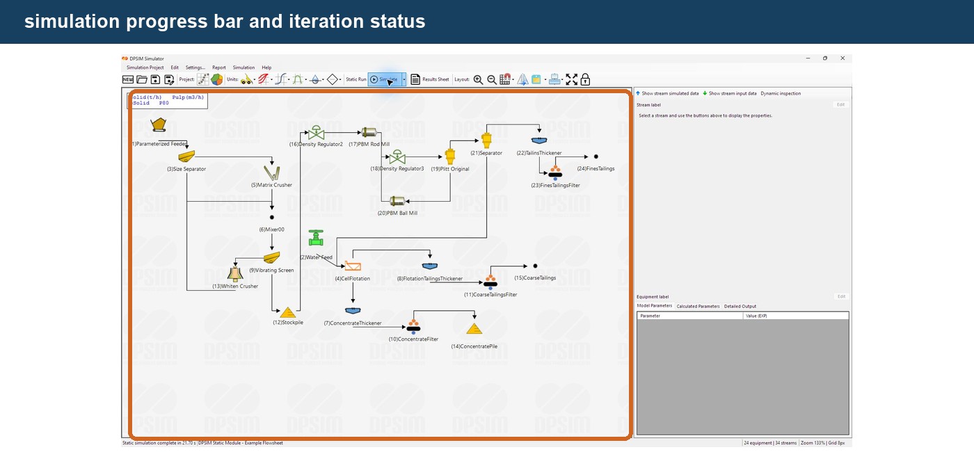
This is particularly useful for larger flowsheets or simulations configured with many iterations.
The interface remains aware that a static simulation is already running and prevents a second static run from being started simultaneously.
Once the calculation finishes, DPSIM refreshes the flowsheet and any open result displays.
Re-running after changing a parameter
One of the main advantages of process simulation is the ability to evaluate alternatives quickly.
Suppose the screen opening is changed from:
1.0 mm
to:
0.8 mm
Open the screen equipment editor, change the parameter and run the static simulation again.
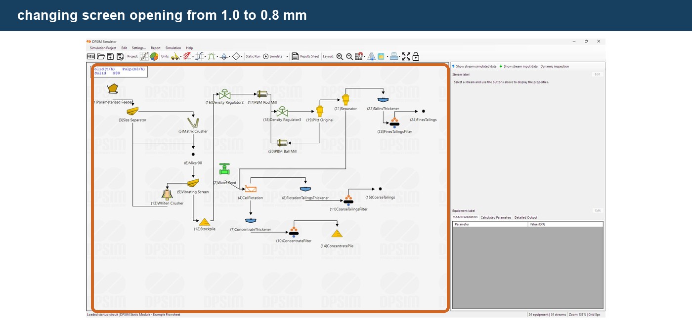
DPSIM recalculates the circuit using the new operating condition.
You can then compare:
Base Case
with:
Modified Case
This workflow can be repeated for:
- equipment settings;
- feed conditions;
- operating parameters;
- model parameters;
- alternative flowsheet configurations.
Changing the feed also requires a new simulation
The same principle applies to the material feed.
Suppose the feed changes from:
1,000 t/h
to:
1,200 t/h
or the PSD becomes coarser.
The process models still contain the previous calculated results until the circuit is recalculated.
Run the static simulation again to propagate the new feed conditions through the flowsheet.
Conceptually:
Change input → Run simulation → Review new results
This should become the normal DPSIM workflow.
What should you check after every simulation?
A successful calculation should always be followed by an engineering check.
Start with the fundamentals.
Mass balance
For a unit with one feed and two products:
Feed mass ≈ Product 1 mass + Product 2 mass
Water balance
If the model does not create or consume water:
Feed water ≈ Sum of product water
Component balance
For each tracked component:
Component in feed ≈ Component in products
PSD
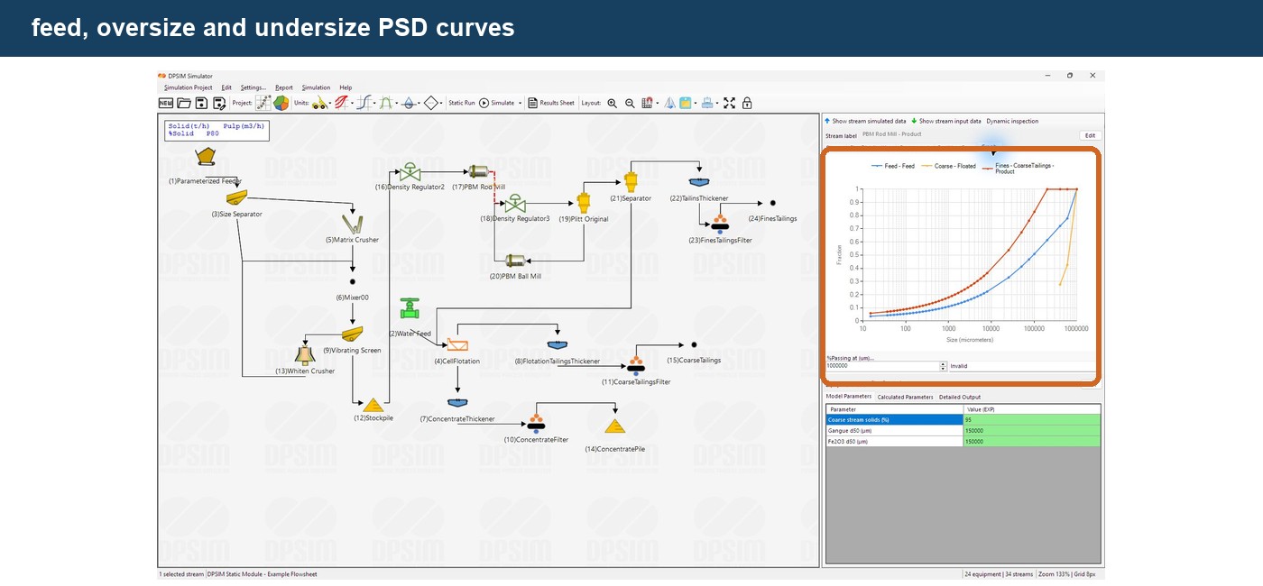
Check whether the resulting particle size distributions are physically reasonable for the process.
For example:
a crusher product should generally be finer than its feed.
Process behavior
Check whether the direction of separation makes sense.
For a screen:
Oversize should be relatively coarse
and:
Undersize should be relatively fine
A simulation result that is numerically calculated is not automatically physically correct.
Start troubleshooting from the flowsheet structure
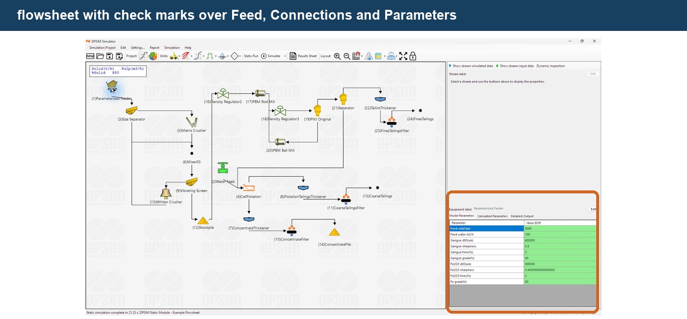
If the simulation produces an unexpected result, begin with the simplest possible checks.
Verify:
Is the feed defined correctly?
Are all required streams connected?
Are the connections going to the correct ports?
Was the intended equipment model selected?
Are the model parameters in the correct units?
Many apparent model problems are actually setup problems.
For example, a stream connected to the wrong product port can produce a mathematically valid but conceptually incorrect circuit.
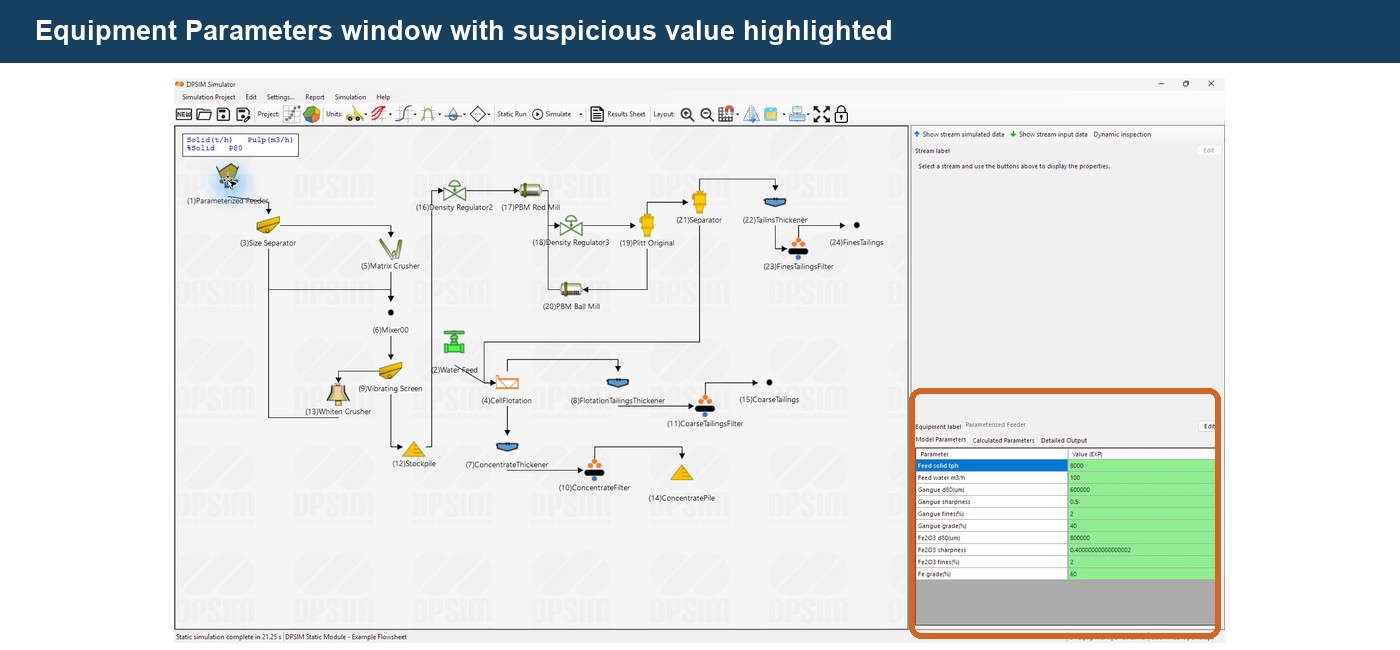
Check the equipment parameters
If the topology is correct, inspect the model parameters.
Look for:
- incorrect units;
- zero values where a positive value is expected;
- unrealistic percentages;
- parameters outside their normal physical range;
- default values that were never replaced;
- component-specific parameters assigned incorrectly.
Compare the parameters with the original engineering source whenever possible.
Do not modify parameters randomly until the model “looks right.”
The objective is to identify the cause of the discrepancy.
Check the material definition
Unexpected results can also originate in the feed.
Verify:
- solids flowrate;
- water flowrate;
- retained PSD fractions;
- component fractions;
- component densities;
- particle size order.
Remember:
DPSIM SizeDistribution is stored in descending particle size order.
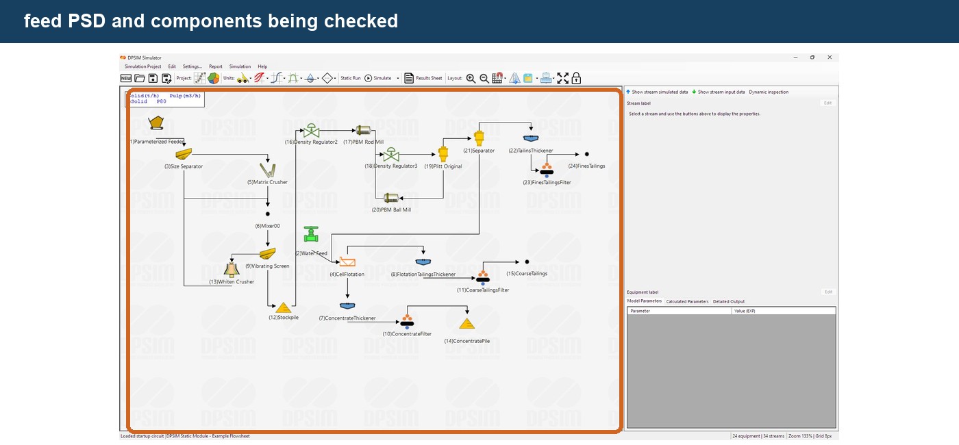
An incorrect feed definition will propagate through every downstream model.
Isolate the problematic unit
For a large flowsheet, troubleshooting the complete circuit at once can be difficult.
A useful strategy is to simplify the problem.
Instead of immediately analyzing:
Feed → Crusher → Screen → Mill → Cyclone → Flotation → Thickener
start by checking:
Feed → Crusher
Then:
Feed → Crusher → Screen
and progressively add the remaining units.
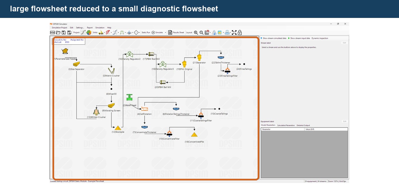
This helps determine exactly where the unexpected behavior begins.
Engineering note
Testing unit models independently is one of the most effective ways to validate a larger simulation.
A complete plant model is only as reliable as the individual process models and data used to construct it.
Be especially careful with recycle circuits
Recycle circuits introduce an additional question:
Has the circuit stabilized?
Consider:
Crusher → Screen → Oversize recycle → Crusher
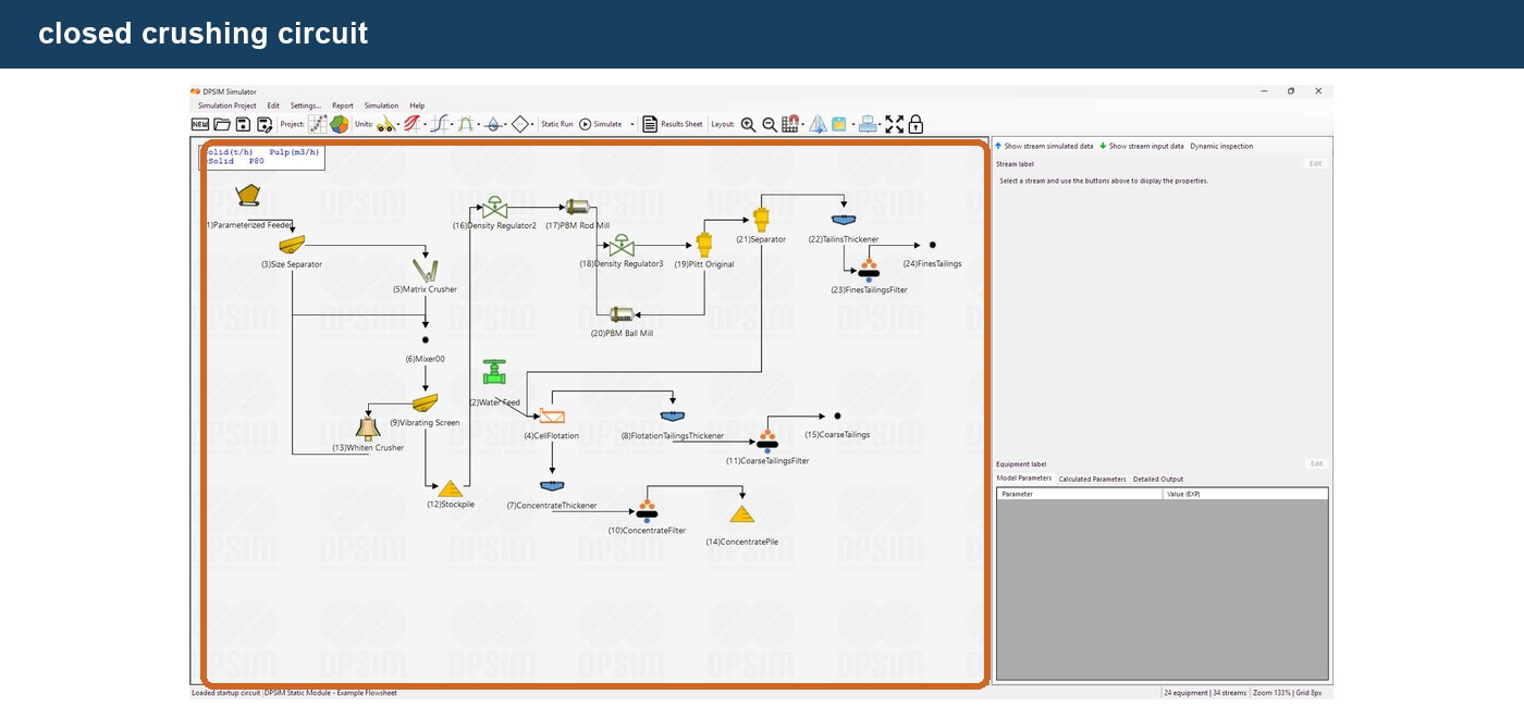
If the recycle changes significantly between iterations, downstream stream results are also still changing.
Before interpreting the final product, verify that the recycle itself has reached a stable condition.
This principle applies to common circuits such as:
- closed crushing;
- ball mill–cyclone circuits;
- regrinding circuits;
- circulating concentration streams;
- water recycles.
A simple first simulation
For the tutorial example:
Editable Feed → Crusher → Screen
run the static simulation.
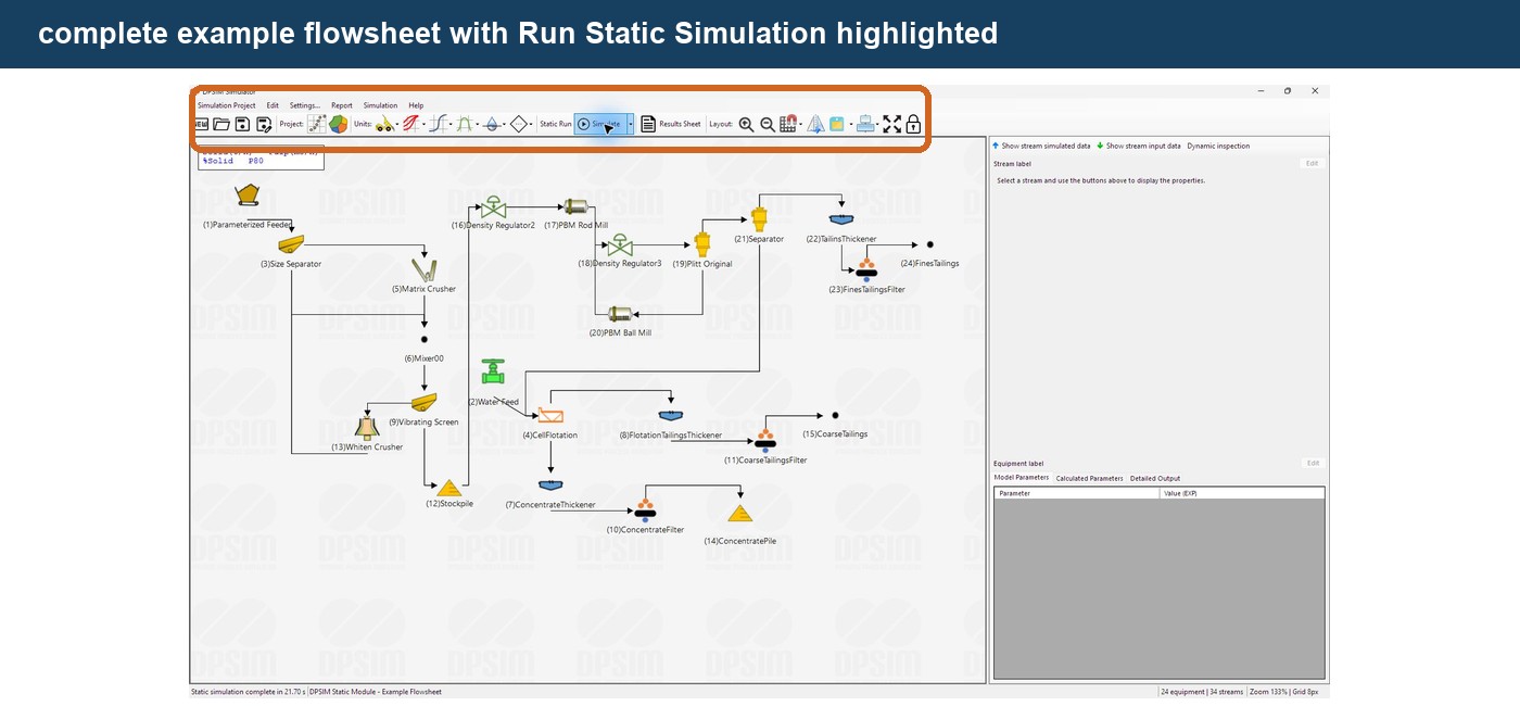
After the calculation:
check the crusher feed and product.
The product PSD should reflect the selected crusher model.
Then inspect the screen products.
The Oversize and Undersize should reflect the classification predicted by the screen model.
At this stage, you do not need to perform a detailed model validation.
The objective is to confirm the complete DPSIM calculation chain:
Feed data
↓
Crusher model
↓
Crusher product stream
↓
Screen model
↓
Oversize and Undersize streams
Our first static process simulation is now complete.
The next question: what did the simulation calculate?
Running the solver is only half of the workflow.
The real engineering work begins when we inspect and interpret the calculated streams.
A DPSIM stream contains much more than total flowrate.
For each stream we can examine quantities such as:
- solids;
- water;
- percent solids;
- densities;
- volumetric flowrate;
- grades;
- P80;
- particle size distribution.
The next tutorial will introduce the Stream Results Sheet and show how to compare calculated streams across the flowsheet.