
Calendar time, exposure, and a production target
Reliability asks whether a specified item or function survives an interval. Availability asks whether it can perform at a specified instant or what fraction of a specified period it is available. Production adds rate, quality, supply, operating policy and calendar. The averages of any two can differ materially. A unit can be available while starved, blocked or operated below its nameplate rate.
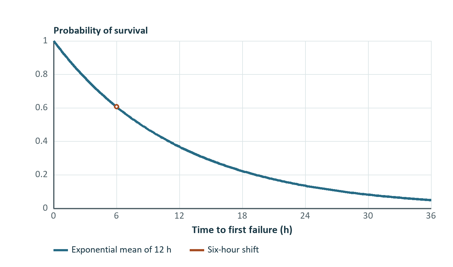
For a repairable unit alternating statistically stationary up periods of mean U and down periods of mean D, the long-run available fraction is U/(U + D). This follows by dividing total accumulated available time by total cycle time and the number of completed cycles. In the simplest active model U = MTBF and D = MTTR with both based on compatible definitions. Here MTBF is the mean up time to failure, excluding the repair period. Exponential operating-time failures with mean U have survival R(t) = exp(−t/U) and constant hazard 1/U. For a two-parameter Weibull lifetime with scale η and shape β, R(t) = exp[−(t/η)^β] and hazard (β/η)(t/η)^(β−1). β = 1 recovers the exponential case. A lifetime clock in operating hours pauses when equipment is inactive. A calendar-time clock continues, as can happen for a site service dependency. Model ageing after repairs consistently with the failure clock.
An independent series pair with U₁ = 90 h, D₁ = 10 h, U₂ = 190 h and D₂ = 10 h has A₁ = 0.90, A₂ = 0.95, and series availability 0.855. At 100 t/h and 8,000 scheduled hours per year, its long-run mean production benchmark is 684,000 t/year when both equipment items are required, material is always available, and throughput is 0 during failures. In a terminating year that begins with both units up and has no historical aging, a simulation can produce a different mean while using the same failure and repair distributions. Shared crews, power interruptions, standby, restart ramps, starvation and feed limitations alter the benchmark assumptions.
Parallel reliability also depends on the performance requirement. If two independent units are each available 90% of the time and each can produce 70 t/h, the probability of at least one being available is 99%. Supplying a 120 t/h demand requires both, so full service probability is 81%. Expected served flow is 0.81 × 120 + 0.18 × 70 + 0.01 × 0 = 109.8 t/h after truncating output at demand. The same two components have three different outcomes for any service, target service, and produced tonnes.
From a state map to an event calendar
A discrete-event model advances to the earliest pending event, integrates any continuous material and performance accumulation to that time, applies a state transition, and schedules its consequences. A transition can be an outage start, restoration, a transport arrival, a buffer becoming empty or full, or a control timer finishing. Between events with constant rates, scalar buffer inventory follows B(t + Δt) = B(t) + (qᵢ − qₒ)Δt. If current B is positive and qₒ > qᵢ, time to empty is B/(qₒ − qᵢ). With qᵢ > qₒ and capacity Bmax, time to full is (Bmax − B)/(qᵢ − qₒ). Recompute that predicted threshold whenever a new state changes either rate. An obsolete event must be cancelled or tagged so that it cannot apply a stale action.
At shared times, tie handling is part of the model. DPSIM orders queued events by time, lower numeric priority, and finally insertion identifier. For example, a replenishment and an empty-buffer event can share a timestamp. Their execution order and the policy validating a threshold determine whether a real downstream trip is recorded. If the model claims an instantaneous zero inventory is sufficient to break a permissive, that transition is deliberate. If it requires a positive interruption duration, reset obsolete empty timers when material arrives. Both cases can close mass while producing different trip counts.
DPSIM's event engine represents entity transfers, queues and resource requests. Long-horizon RAM modeling can include repair resources, spares, dependencies, degraded capacity, common-cause states, standby and preventive maintenance. Its hybrid material inventory can advance continuous rates analytically between events. Rate-to-batch and batch-to-rate interfaces represent the event and process sides of transport. Detailed equipment may also use a fixed-step model, so integration of fleet events with detailed particle populations depends on which adapters and state boundaries are present. A bounded experiment should preserve reproducible streams for individual stochastic sources. DPSIM uses a PCG family generator and derives streams from the experiment and replication identifiers. O’Neill, 2014
Worked event trace
A crusher outage lasts from 0 to 3 h. A downstream process requests 80 t/h and can draw from a buffer containing 120 t at t = 0. The buffer holds at most 160 t. On restoration, input rises to 100 t/h until the buffer reaches capacity. At capacity, the assumed upstream throttle matches demand.
| Time interval (h) | Feed (t/h) | Product (t/h) | Start stock (t) | End stock (t) | Unserved demand (t) |
|---|---|---|---|---|---|
| 0 to 1.5 | 0 | 80 | 120 | 0 | 0 |
| 1.5 to 3 | 0 | 0 | 0 | 0 | 120 |
| 3 to 11 | 100 | 80 | 0 | 160 | 0 |
| 11 to 12 | 80 | 80 | 160 | 160 | 0 |
The stock covers 120/80 = 1.5 h of the outage. Once restored, net fill is 20 t/h and requires 8 h. Total received mass is 880 t and produced mass is 840 t, so 120 + 880 − 840 = 160 t remaining. Requested mass is 960 t over 12 h. The downstream process supplies 87.5% of demand despite upstream availability of 75% over the same period. These are trace-specific figures. If the plant throttles differently, uses the starting inventory elsewhere, or restarts slowly, timing and tonnes have to be recomputed. A finite annual simulation also credits any remaining stock according to a declared accounting basis rather than treating it as product.
Replications, uncertainty, and evidence
A terminating experiment typically asks for production during a specific mine year, campaign, or shift. Set the initial inventories and equipment states to match the inference. For an equilibrium-average question, consider an initial warm-up excluded from the measured period and assess whether start-up transients still influence outcomes. Replications must be independent when using conventional replication-based standard errors. The individual daily or hourly records inside one replication are serially dependent, partly because failures and buffer inventories persist.
Let Yᵣ be the produced mass of replication r, with n replications. For sample mean Ȳ and sample standard deviation s, a two-sided approximate confidence interval for the model mean is Ȳ ± t₁₋α/₂,ₙ₋₁s/√n. Five illustrative yearly outcomes of 670, 683, 696, 685 and 686 kt give Ȳ = 684 kt and s = 9.301 kt. With t₀.₉₇₅,₄ = 2.776, the 95% interval is 672.45–695.55 kt for the model mean. A production quantile describes the variability in individual years. Its estimate requires far more support in its tail than these five outcomes provide. Estimating an expected difference between two interventions can use matched stochastic source streams and a confidence interval on the paired differences. For adaptive replication, define the acceptable interval half-width and maximum run count before evaluating alternatives. Welch, 1982, on simulation steady-state output analysis
Historical records should identify exposed operating hours, outages already ongoing at the observation boundary, time in degraded service, work waiting for parts or personnel, and any stopped intervals excluded from the KPI. Discarding censored intervals can bias failure estimates toward short lifetimes. Fitting reliability distribution shapes to sparse data supplies uncertainty as well as a curve. Use controlled cases to verify availability for a single unit, the independence limit for a series path, conservation for an inventory trace, and the same replay for the same seed. Use historical throughput and interruption-duration data to test the coupled plant forecast.
Exercises with answers
- An exponentially failing unit has mean up time 200 h and mean repair time 10 h. Find mission survival over 24 h and the long-run available fraction. Answer. exp(−24/200) = 0.8869, while A = 200/210 = 0.9524.
- In the event trace, raise starting stock to 180 t and capacity to 200 t. Assuming fresh input still resumes at 3 h, find time to empty and unserved demand. Answer. Empty at 180/80 = 2.25 h. Unserved mass is (3 − 2.25) × 80 = 60 t.
- If a nominal 95% half-width is 12 kt with 25 independent replications, estimate replications for 6 kt with similar variance and a nearly constant critical value. Answer. Standard error scales as 1/√n, so roughly 100 replications.
- What changes when two units with individually independent failure modes share a single repair crew? Answer. Component up/down histories become dependent through queueing and the effective downtime includes crew waiting. The product availability formula using isolated-unit means no longer supplies the production benchmark for that staffing policy.