
The duty precedes the model
Size reduction is expensive because it changes an entire distribution of particles while the rest of the plant often responds to a narrow portion of that distribution. A coarse fraction may govern crusher recycle, while a fraction near a mineral liberation size may control flotation. Material much finer than the liberation size may consume grinding power and depress recovery. Thus a duty statement such as “make an 80 µm product” is incomplete. A usable statement specifies the dry solids throughput, the feed and product percentile or full size distribution, the motor or shaft power boundary, and the process downstream that benefits from the size change.
Define F80 and P80 as the sizes below which 80% of the feed and product dry mass, respectively, pass. These are properties of streams and are evaluated from their cumulative dry-mass size distributions. A classifier d50 is the size at a specified partition probability, so it measures a different quantity. Confusing P80 with d50 imposes a target on the wrong stream and may lead to a numerically consistent design that cannot meet the process duty.
When only widely spaced sieve measurements are available, specify the percentile interpolation convention. If passing fractions p₁ and p₂ bracket a desired passing fraction p at apertures x₁ and x₂, the following equation interpolates linearly in log size.
A percentile below the smallest measured aperture or above the largest one must be treated as bounded or estimated by a stated fitted tail. This choice matters in energy calculations because the difference between reciprocal size terms can be small and sensitive to errors in either percentile.
Energy laws and their units
A convenient historical family describes the differential size reduction duty as proportional to an inverse power of characteristic size x.
The sign makes energy positive during size reduction. Setting n = 1 gives a logarithmic Kick-type dependence on the size ratio. Setting n = 2 gives a Rittinger-type dependence on the difference between inverse sizes. For similar particle shapes and a single characteristic size, the inverse size is proportional to surface area per unit mass. The intermediate n = 1.5 gives a Bond-type square-root dependence. Actual ores and mills have selection, breakage, transport and rheological effects that this one-dimensional family cannot separate. Use a fitted energy law over the size and operating range where it was calibrated.
The engineering Bond expression uses the feed and product square-root size terms.
Here F80 and P80 are numerical values in µm, E is specific energy in kWh per tonne of dry solids, and Wᵢ must be expressed on the same tonne basis. The numerical coefficient includes the µm convention. A work index reported per short ton requires conversion to the intended mass basis before use. A laboratory value belongs to its specific material and test procedure. Any correction for device efficiency or a comparison between shaft and net grinding power is an additional assumption.
P is power in kW on the chosen measurement boundary and Qₛ is dry solids flow in t/h on the matching stream boundary. For example, dividing motor input power by slurry flow changes both the energy numerator and its solids basis. In a closed circuit, power per tonne of fresh feed and power per tonne of mill feed also differ, because the second denominator includes circulating load. Both can be useful when labelled precisely.
Worked power and capacity calculation
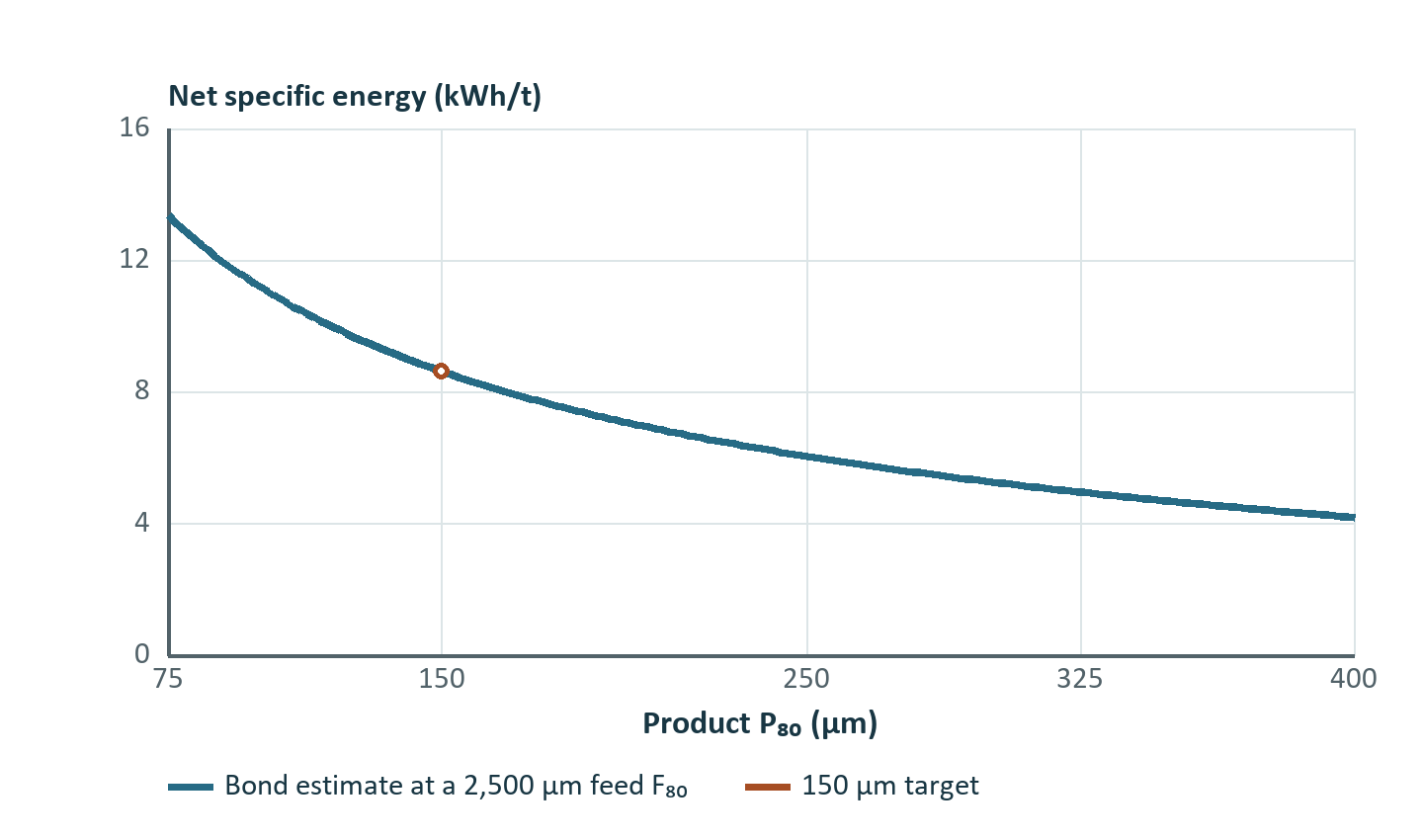
A mill is assessed at 250 t/h dry solids with F80 = 2500 µm and P80 = 150 µm. The applicable metric work index is 14 kWh/t. These inputs give the following net specific energy.
The corresponding net duty is approximately 2158 kW. If measured electrical input is 2410 kW at the same point, its specific energy is 9.64 kWh/t. The ratio of calculated net duty to electrical input is about 0.895 for this comparison. This number combines any power-boundary difference and the error of the energy model. It cannot identify a gearbox, motor or grinding efficiency individually.
Suppose available power on the net boundary falls to 1800 kW and throughput remains fixed at 250 t/h. Then E = 7.2 kWh/t. Rearrange the same fitted relation to solve for P80.
The resulting P80 is approximately 196 µm. If the process instead requires 150 µm, the corresponding energy-limited throughput is about 209 t/h at 1800 kW. A hydraulic or discharge capacity limit could reduce the feasible throughput further. The calculation thus offers two operating alternatives at fixed energy calibration, each with a distinct impact on the downstream process.
Complete distributions from sparse specifications
A known-product model imposes a supplied PSD while calculating power or simply transporting the mass. It is a reasonable representation of a crusher covered by a supplier test, a grinding unit whose measured product is held fixed in a plant balance, or a boundary stream imported from a pilot study. Its predictions outside the test conditions come from the additional assumptions used to vary the product curve. A target P80 model imposes one percentile. An available-power model can instead estimate which P80 is attainable, given a feed, throughput and energy calibration. These alternatives exchange which information is constrained and which is predicted. In Available Power Comminution, specified power and actual dry feed determine specific energy and the product-size duty. In Specific Energy Comminution, a fixed operating energy per tonne makes required power proportional to throughput. Known P80 Comminution specifies a product percentile and estimates the corresponding power. Rosin–Rammler Product Comminution describes one product population, and Bimodal Rosin–Rammler Comminution resolves two weighted populations.
A Rosin–Rammler size curve parameterized by a specified percentile P80 and positive shape parameter n gives the following cumulative passing function.
F(x) is the cumulative dry-mass passing fraction at aperture x, with x and P80 in the same units. Larger n makes the curve steeper at its characteristic size. All such curves pass exactly 80% at P80. For x below P80 the fraction passing falls as n increases. For example, with P80 = 150 µm at aperture 75 µm, n = 1 gives 55.3% passing while n = 2 gives 33.1%. An energy calculation using only the common P80 would see the same duty in these two products. A downstream process sensitive to the minus-75 µm fraction receives substantially different feed.
A bimodal product curve is a weighted sum of two cumulative curves, such as a primary grinding population and a population of already fine material. Let w be the dry-mass fraction assigned to the first mode.
The mixture percentile is the root of F_total(x) = 0.8. Averaging the individual P80 values does not generally locate this root. Set w on a mass basis and constrain its fitted range to [0,1]. When only one or two sieve points are available, several combinations of mode sizes, shapes and weights may give the same observed curve. In that case report a constrained or scenario fit. A carefully chosen parametric assumption can support a design comparison even when its individual coefficients are unidentifiable.
Calibration and interpretation
Use measured feed and product distributions from synchronized operating periods. Fit power against the same time interval and stream throughput used to calculate the percentiles. For a trial relative error in measured power or mass flow, E = P/Qₛ implies approximately ΔE/E ≈ ΔP/P − ΔQₛ/Qₛ for small changes. A 5% throughput bias can therefore resemble a change in material hardness. In a blend, fit composite behaviour only if ore variability, media and load are sufficiently controlled. Include mineralogical measurements or separate testwork when those factors vary. Replicate critical cases at materially different F80, feed rates or mixed fractions to distinguish an interpolating fit from a robust prediction.
Compare both percentile and full-distribution errors. When the root of an inverse energy calculation requires a target finer than the calibrated data or demands negative grinding energy because P80 exceeds F80, inspect the process boundary, measurements and model. The device may be primarily classifying, feeding blended material, or operating on a broken power assumption. A size-reduction energy law is suitable once the observed size change is attributable to breakage on the chosen boundary.
Exercises and solutions
- A device draws 1000 kW net at 125 t/h dry solids. Feed and product have F80 = 800 µm and P80 = 100 µm. Find the fitted metric work index on this operating point.
- Two product populations at 75 µm have passing fractions of 0.30 and 0.80. The coarser population contributes 60% of the dry mass. Find total passing at 75 µm.
- One mill handles 300 t/h total solids, of which 120 t/h is incoming recycle. Net shaft duty is 2700 kW. Report specific energy on mill feed and fresh feed.
Solutions. (1) Net energy is 8.0 kWh/t. Wᵢ = 8/[10(1/√100 − 1/√800)] = 12.38 kWh/t. This is an operating estimate under the fitted model. (2) Total passing is 0.60 × 0.30 + 0.40 × 0.80 = 0.50. (3) Mill feed specific energy is 9.0 kWh/t and fresh feed specific energy is 2700/(300−120) = 15.0 kWh/t. Use the circuit boundary consistently when comparing either figure with a design reference.
Selected references. Bond (1952), third theory of comminution. Charles (1957), energy-size relationships. Morrell (2008), energy requirements and utilisation efficiency for comminution circuits.