
A measured sieve vector can be the most direct feed specification for a single plant condition. Parametric distributions provide a compact description when comparing different ore domains, filling modest measurement gaps or studying sensitivity at a proposed operating point. The choice is a modeling claim about curve shape. A parameter shared across ore domains is evidence of transfer only if the new data confirm it. A long extrapolation from a narrow sieve window should carry uncertainty from the chosen distribution family as well as the fitted coefficients.
Let x be a positive equivalent particle size and F(x) the dry mass fraction passing. Define the sorted size cuts before sampling any analytic curve. For every bounded interval compute the difference of successive F values. Add the open ends with the measured or assumed distribution support. For a continuous curve, calculating an interval fraction from the density at a representative size times the interval width is an approximation. Direct differencing of the cumulative formula is exact within that description and is usually inexpensive.
Gaudin–Schuhmann
A capped power law is a convenient description over a wide size range when a log–log plot of cumulative passing is approximately straight below the top size X. Its parameters are the positive shape m and top scale X.
Two uncensored measurements x₁ < x₂ with 0 < F₁ < F₂ < 1 imply m = ln(F₂/F₁) / ln(x₂/x₁), then X = x₂ / F₂^(1/m). Lower x values with zero recorded counts are left-censored and need care in a log fit. A point with 100% passing reports a constraint on the top range of the sample. A series of such points above X should not be used to flatten the estimated slope.
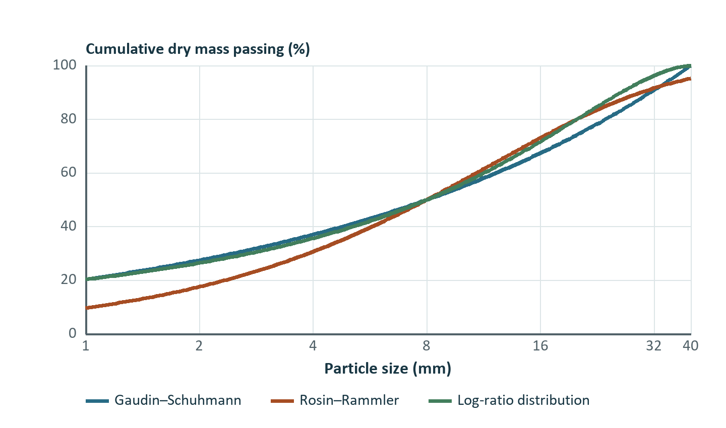
For measurements of 25% passing 4 mm and 50% passing 8 mm, m = 1 and X = 16 mm. Estimated passing at 2 mm is 0.125 and at 12 mm 0.75. At 80 t/h the mesh of 16, 8, 4 and 2 mm yields zero >16 mm, 40 t/h at 8–16 mm, 20 t/h at 4–8, 10 t/h at 2–4 and 10 t/h below 2. The model implies a hard top support. If a sparse photograph captures occasional 35 mm fragments in the same material, the capped law can still fit the central percentiles but requires reconsideration for a grizzly or conveyor transfer design.
Rosin–Rammler
The Rosin–Rammler passing function uses a scale a and positive shape n. It has unbounded upper support in its conventional mathematical form.
At a, the cumulative passing is 1 − e⁻¹ ≈ 0.632121. When using d₈₀ as the scale of a parametrization, write the exponent as −ln(5) (x/d₈₀)ⁿ. The point at d₈₀ then passes exactly 80% before any correction. If a material feed model embeds an unresolved fines fraction f₀, a useful form is f₀ + (1 − f₀) [1 − exp(−ln(5)(x/d₈₀)ⁿ)]. This law treats f₀ as an offset allocated at the fine end. At the entered scale d₈₀ the total passing is 0.80 + 0.20 f₀. An engineer seeking exactly 80% total cumulative passing must account for the offset.
A convenient diagnostic plot uses ln[−ln(1 − F)] versus ln x. The theoretical slope is n. Points close to zero and one are unstable after transformation, so inspect the residuals in original mass terms. First fit from useful points with 0 < F < 1, then verify against actual retained mass per class. When multiple size percentiles are known, for n from two inputs q₁ and q₂ the numerator is ln[−ln(1 − q₂)] − ln[−ln(1 − q₁)], and the denominator is ln(x₂/x₁).
For x₅₀ = 4 mm and x₈₀ = 9 mm, n ≈ 1.039 and a ≈ 5.69 mm. At 2 mm the estimated passing is about 0.286. At 16 mm, roughly 5.4% remains above the aperture. For a measured screen product with a demonstrated 16 mm top size, that excess suggests either a hard cut representation or a truncated curve normalized at a justified upper limit. Truncation changes all passing fractions; clipping at an upper size without renormalizing below creates an abrupt mass concentration at the cutoff.
Log-ratio particle size distribution
For a positive top size X, median m and positive shape b, the log-ratio distribution expresses passing using logarithmic distance from the top. It approaches zero toward vanishing size, passes half at m, and attains one at X.
A second implementation calculates the shape from the size measured at 80% passing, s, after receiving X and m. At s we have zᵇ = 0.25. Thus b = ln(0.25)/ln[ln(X/s)/ln(X/m)]. The required order is 0 < m < s < X. When s is very close to m, the denominator approaches zero and small shifts in the two measurements can strongly alter b. When s approaches X, b tends toward zero. In both cases verify the inferred tail against at least one withheld point.
Suppose the measured top size is 40 mm, x₅₀ = 8 mm and x₈₀ = 20 mm. The ratio z at x₈₀ is ln 2 / ln 5 ≈ 0.43068, and b ≈ 1.645. For x = 4 mm, z = ln 10 / ln 5 ≈ 1.43068 and passing is about 35.7%. At 2 mm passing is about 26.4%. At X, the exact fraction is one by definition. On an 80 t/h feed, the difference between 50% and 35.7% gives about 11.4 t/h in the 4–8 mm interval. If independent sieving shows only 20% passing at 4 mm, the three anchor quantities constrain a curve that misses a critical fine region. A tabulated PSD or separately characterized population blend is then warranted.
Ouchterlony (2005) introduced the log-ratio distribution in the fragmentation-distribution literature. The form above models the measured size population reaching a plant study boundary. It is most directly checked using independent sieve or particle characterization data on that population. The two private implementations in DPSIM carry a common component grade vector across size for these parametric feeds. It represents a separable joint model in which the declared PSD has the same shape for each material component. Feed-specific mineral assays by size provide a test of that simplifying assumption.
Component-specific distributions and blends
An ore containing a soft weathered component and a resistant primary component can show a curved log–log distribution that a single parametric family fits poorly. A blend gives independent marginal distributions in each component. With dry feed grade g꜀ and cumulative P꜀(x) for component c, the total passing is Σ g꜀ P꜀(x). In class i, the dry flow of that component is S g꜀ [P꜀(uᵢ) − P꜀(lᵢ)]. Divide by the total class flow to compute the grade in that size class. The calculation explains why a geographically small fraction of weathered ore can dominate ultrafine material.
| Material | Fraction of total dry solids | Passing 250 µm | Contribution to feed passing |
|---|---|---|---|
| Weathered material | 0.25 | 0.70 | 0.175 |
| Primary material | 0.75 | 0.10 | 0.075 |
| Total | 1.00 | — | 0.250 |
Weathered ore is 25% of total dry solids and 70% of the material below 250 µm. Above that point it is just 0.075/0.75 = 10% of dry mass. If independent assays show the weathered component carries a penalty mineral, estimating a penalty based on bulk blend proportions alone could severely underpredict its grade in a fine product. The component PSD feeder in DPSIM implements an analogous construction with parametrized passing curves, a fines offset and additive dry component masses. The batch feeder uses analogous population inputs on an amount-based boundary for batch studies. Water and solid batch amounts must be assigned consistently to the chosen cycle or time basis before connecting them to throughput estimates.
Variable feed boundaries
A variation of throughput and size can be supplied as independent series, a campaign sequence or a joint conditional model. Suppose observed reclaim at higher rates generally has a finer feed owing to how an ore domain is scheduled. Independently sampling throughput and PSD generates scenarios that break this observed dependence. In a closed grinding circuit the effect may appear as unrealistic simultaneous high loading and coarse feed. For a counterfactual investigation it can be useful to impose such a joint stress point. Label it as a design scenario.
Variable PSD feed control distinguishes physical composition from the numerical representation of changes in size. If blending between two end-member feeds with flow rates Sₐ and Sᵦ and passing curves Fₐ, Fᵦ, use (SₐFₐ + SᵦFᵦ)/(Sₐ + Sᵦ) at every size. Interpolating percentiles between the two curves gives a different result because percentiles are inverses of the distribution. Across a step change, any transport delay belongs to conveying or residence time. A variable feed boundary describes the rate and distribution that cross the specified location at the stated time.
Exercises with solutions
Exercise 1. An offset Rosin–Rammler curve has f₀ = 0.10, scale x₀ = 500 µm for the 80% passing point of the fraction outside the offset, and n = 1.3. Find the size at which the total feed has 80% passing.
First solve for the passing fraction of the main population, (0.80 − 0.10)/0.90 = 0.77778. The scale correction is [−ln(0.22222)/ln(5)]^(1/1.3). The total d₈₀ is about 475 µm. At 500 µm the total cumulative passing is 82%.
Exercise 2. A 60 t/h feed model allocates the same size curve to several minerals. It has 10% valuable mineral and 25% passing 250 µm. A plant survey finds 18% valuable below that size. Compute the implied valuable grade in the rest of the feed.
The fine stream carries 15 t/h dry mass and 2.70 t/h valuable mineral. The bulk feed carries 6.00 t/h valuable mineral, leaving 3.30 t/h in the remaining 45 t/h. Coarse grade is 7.33%. A uniform grade simulation would place only 1.50 t/h valuable in the fines and misallocate 1.20 t/h.
Exercise 3. A feed has a measured median of 8 mm and an inferred top size of 40 mm. Compare the d₈₀ obtained by the capped power law with m fitted to the median, and the measured-percentile log-ratio example.
For the power law, m = ln(0.5)/ln(8/40) ≈ 0.43068. The predicted d₈₀ is 40 × 0.8^(1/m) ≈ 23.83 mm. The log-ratio example gives 20 mm by its measured anchor. A withheld point around the upper-central range is informative about the family choice when median and top support alone are available.