
A steady mineral-processing flowsheet combines material-balance equations, unit equations and operating specifications. The flowsheet graph determines both physical connectivity and the computational order. Serial units can be evaluated once when their inputs are known. A recycle creates a circular dependence between calculations. The engineering problem is to find a common set of stream states satisfying the conservation laws and the unit calculations.
From a network to a solve
Represent flows in conserved coordinates: dry solids, water, component masses and size-by-component masses when the data support them. Derive mass fractions, grade, density and percent solids from their reconciled rates. Mixing volume percentages or normalized size distributions directly gives the wrong mass basis whenever streams carry different solids concentrations.
For an open graph, process nodes in a topological order. A strongly connected component is a maximal region in which each node can reach all the others. A region that includes a circuit loop requires simultaneous solution or a numerical tear. Cutting a recycle stream computationally creates an assumed inlet state at one end and a calculated return at the other. Physical material remains in the original loop. For an estimate x of tear rates and one sweep of unit models T, use
Specifying both a fixed cyclone feed flow and an independent fixed fresh solids feed to a circuit with recycle may overconstrain it. Count free specifications, check active capacity and control constraints, and examine the residuals. A missed split specification can leave many feasible fixed points. A conflicting target can leave none. Neither condition is diagnosed reliably by iteration count alone.
Direct substitution, scaling and acceptance
The simplest calculation is xₖ₊₁ = T(xₖ). In a differentiable region near the solution, eₖ₊₁ ≈ Jₜeₖ. Local direct convergence requires the linearized error modes to decay; a sufficient local criterion is spectral radius less than one under standard smoothness conditions. In a scalar linear example the derivative gives the exact geometric convergence factor. In multi-stream loops, changing one source may excite several interacting modes even if the total dry flow appears stable.
A physically meaningful residual test scales rates by absolute and relative tolerances. For variable i define
The absolute term uses the units of the variable and sets the noise floor near zero. The relative term preserves numerical discrimination at high flow. A typical scaled acceptance test requires maxᵢ sᵢ ≤ 1 over more than one successive pass. Monitor water, dry solids and meaningful size and component rates. A loose tolerance on the only valuable component in a trace metal circuit can leave an important metallurgical error hidden by closure of total dry flow. Use a separate component floor consistent with its measurement basis and decision. After convergence, run external balances and unit constraint checks as independent tests. Tiny changes between iterates can occur at a clamped constraint or an abandoned branch even when the original equations remain unsatisfied.
Worked example: a scalar circulating load
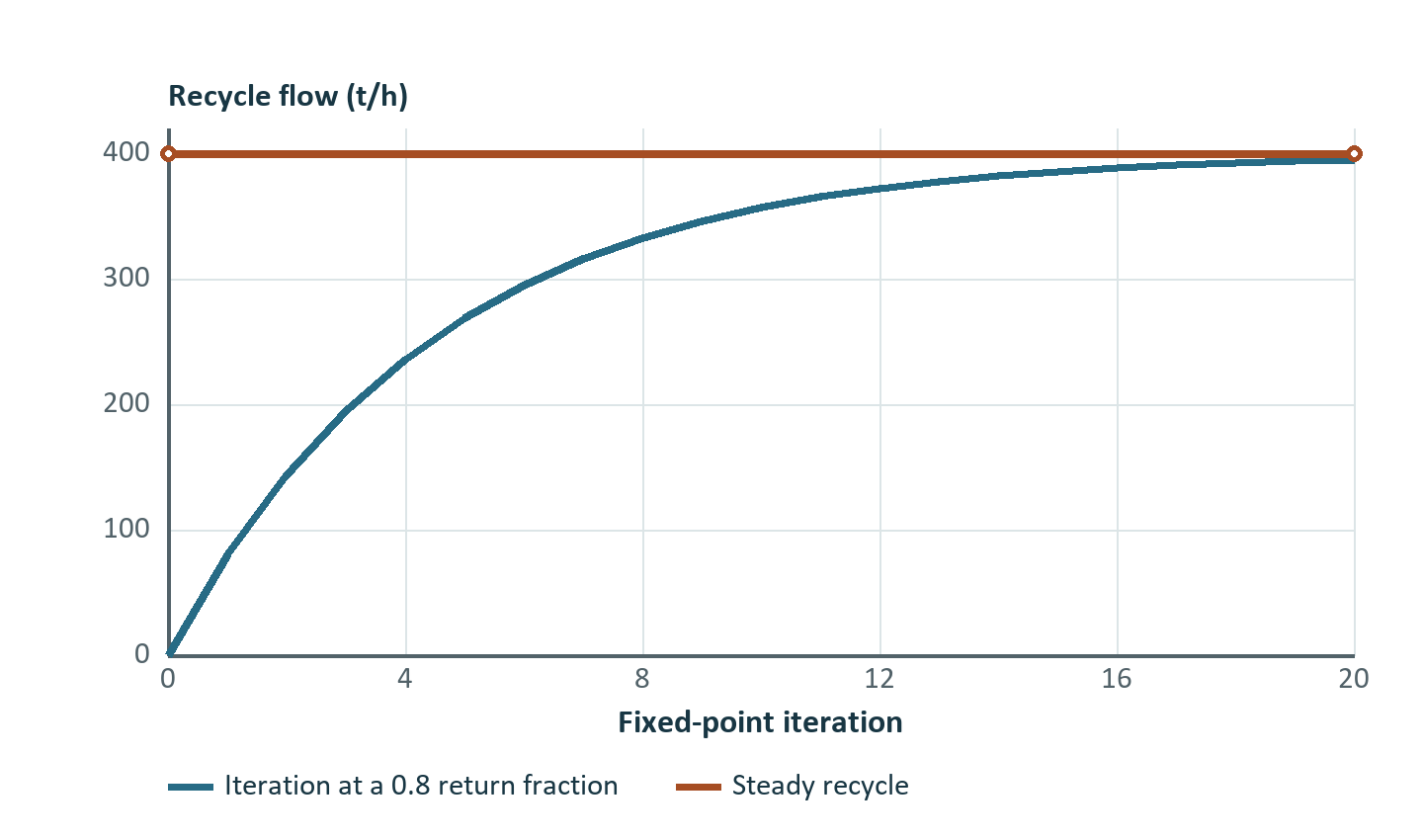
Suppose 60% of dry solids sent around a mill–classifier loop returns as recycle. Fresh solids feed is 100 t/h. At steady state,
The mill feed is 250 t/h and final product is 100 t/h. Circulating load is 150% on fresh dry solids feed. It would be 60% on total mill feed. The denominator should accompany the percentage.
| Pass | Recycle sent into pass (t/h) | Calculated return (t/h) | Difference (t/h) |
|---|---|---|---|
| 1 | 0.000 | 60.000 | 60.000 |
| 2 | 60.000 | 96.000 | 36.000 |
| 3 | 96.000 | 117.600 | 21.600 |
| 4 | 117.600 | 130.560 | 12.960 |
| 5 | 130.560 | 138.336 | 7.776 |
After k completed updates the error magnitude is 150 × 0.6ᵏ t/h. Increasing the loop return to 98% at unchanged fresh flow gives a formal solution of 4,900 t/h recycle and a factor of 0.98. More passes can shrink the residual slowly, but the formal result may exceed mill, pipe and cyclone capacity. This is an operating feasibility question as well as a numerical one. At unit gain with positive fresh feed the assumed steady circuit has no finite solution.
Relaxation and acceleration
With scalar relaxation xₖ₊₁ = xₖ + ω[T(xₖ) − xₖ], the local multiplier is 1 − ω + ωT′. If T′ = −1.2, choosing ω = 0.5 yields −0.10 and damps an alternating iterate. If T′ = 0.98 and ω = 0.5, the factor becomes 0.99, slowing an already stable monotonic approach. Therefore a damping parameter should be connected to the observed behavior.
A scalar secant prediction uses two estimates of the actual residual F and solves its local line for zero:
For the affine recycle example this line finds the solution directly once two distinct residuals are available. Similar ideas underlie Wegstein acceleration and multidimensional fixed-point accelerators. Reject excessively large trial steps and fall back to a safeguarded pass when the denominator is small, expected material rates become negative or an equipment capacity branch changes. Re-evaluate original residuals at every proposed accepted point. Wegstein, 1958 Anderson, 1965
For a vector residual, Newton linearization solves J_FΔ = −F. Jacobian estimates can be expensive for a whole process network and unreliable across event guards or active constraints. Sparse structure, sectioning, trust regions and continuation on operating conditions help. Try solving an easier physical circuit with modest recycle and increase it gradually when starting guesses are poor. Detect invalid specifications or violations of plant limits before investing in an expensive solver.
Convergence near a threshold and with dynamic boundaries
Capacity clamps and switching logic change which equations are active. A valve or downstream route can repeatedly alternate states if the previous iterate alone determines the decision near its threshold. Inspect which state is oscillating. A physically specified deadband or state rule may change the model into a well-defined representation. Arbitrary averaging of states obscures the operating limit. A switch held constant within a steady solve can be evaluated separately on each feasible branch. If both branches are admissible, the application may need explicit operating logic or a dynamic initial condition to decide which branch is reached.
A recycle through a true material inventory may be causal instead of instantaneous on a time step. A stockpile discharge determined by an already accepted inventory state provides a known boundary for the current algebraic solve. Rate reconciliation closes for that frozen boundary. The next state is advanced from the material balance afterward. DPSIM's hybrid stationary solver implementation documents this distinction. It computes dependency regions to identify algebraic cycles, uses a global fixed-point calculation in the hybrid solve, and reports residuals combining solids, water, size and component masses. This is distinct from authoring tools that support explicitly specified fixed-iteration steady runs. Use the matching diagnostics for the calculation being evaluated. DPSIM Developer reference
Exercises and answers
- A recycle is 75 t/h and fresh solids are 125 t/h. Compute circulating load on fresh feed and recycle fraction on total unit feed. The values are 60% and 37.5%, respectively.
- For absolute tolerance 0.02 t/h and relative tolerance 0.001, would a change from 100 to 100.04 t/h pass a single-variable scaled test? The denominator is 0.12004 t/h and the scaled residual is about 0.333. This variable passes. Other variables and consecutive-pass rules still apply.
- A 1,000 t bin's dispatch is fixed over a calculation step by an independently advanced inventory model. Should its outgoing material be solved from the current inflow as an algebraic equality? Its outgoing rate is a boundary supplied by the dispatch state for that step. The inflow–outflow difference advances the inventory.