Our project now contains a defined material feed.
We know:
- how much solid enters the process;
- how much water enters;
- the particle size distribution;
- the solid components;
- the composition of each particle size class.
The next step is to define what happens to that material.
In DPSIM, process operations are represented by equipment objects placed on the flowsheet. Each equipment object is associated with a mathematical model that determines how its incoming material streams are transformed into its output streams.
In this tutorial, we will explore the DPSIM process model library and add our first process equipment to the flowsheet.
In this tutorial you will learn how to:
- understand the DPSIM equipment categories;
- distinguish the graphical equipment object from its process model;
- select a model from the toolbar;
- add equipment to the flowsheet;
- understand equipment input and output ports;
- organize and identify process units;
- choose an appropriate model for the objective of the simulation.
| DPSIM equipment categories |
|---|
 |
| From left to right: Feed, Comminution, Classification, Concentration, Dewatering and Auxiliary. |
Figure 1. DPSIM toolbar with the main equipment categories highlighted.
The DPSIM process model library
The DPSIM Static Module organizes available models into six main categories:
Feed
Comminution
Classification
Concentration
Dewatering
Auxiliary
| Equipment categories | Equipment categories | Equipment categories | Equipment categories | Equipment categories | Equipment categories |
|---|---|---|---|---|---|
| Feed | Comminution | Classification | Concentration | Dewatering | Auxiliary |
| • Editable Product Stream Feed | • Crushers • Mills • HPGR | • Screens • Hydrocyclones | • Flotation • Separators | • Thickeners • Filters | • Mixers • Splitters |
Figure 2. Toolbar showing Feed, Comminution, Classification, Concentration, Dewatering and Auxiliary.
Each category is divided into smaller groups according to the type of process operation.
For example, Comminution includes groups such as:
- Crushers;
- Mills;
- HPGR;
- Product size;
- Energy.
Classification includes:
- Screens;
- Hydrocyclones;
- Partition curves.
Concentration includes models for operations such as:
- Flotation;
- Separators;
- Gravity separation and other concentration methods, depending on the installed model set.
Dewatering includes operations such as:
- Thickeners;
- Filters.
And Auxiliary contains operations that support the construction of the flowsheet, including:
- Mixers;
- Splitters;
- Buffers;
- material handling models;
- other auxiliary functions.
| Examples of expanded categories | Examples of expanded categories | Examples of expanded categories |
|---|---|---|
| Comminution | Classification | Auxiliary |
| • King Primary Crusher • Whiten Crusher • PBM Ball Mill | • Karra Screen • King Screen • Plitt Hydrocyclone | • Mixer • Multi-output Splitter • Static Pile |
Figure 3. Examples of two or three expanded equipment categories.
This organization makes it easier to find models according to their process function rather than searching through a single long list.
Equipment and mathematical models
An important concept in DPSIM is the relationship between the equipment shown on the flowsheet and the mathematical model behind it.
Consider a crusher.
On the flowsheet, the crusher appears as a graphical process unit:
Crusher icon
But the icon alone does not determine how the crusher behaves.
Its behavior comes from the mathematical model associated with that equipment instance.
For example, the DPSIM comminution library contains different crusher modeling approaches.
These models may use different parameters, assumptions and equations to predict the resulting product size distribution.
| Crusher models with different equations | Crusher models with different equations |
|---|---|
| Matrix models | Selection criteria |
| • Generic Matrix Crusher • Whiten Crusher • Modified Whiten Crusher | • Available input data • Required parameters • Validation range |
Figure 4. Two crusher model entries with similar process function but different model names.
Therefore:
Process equipment = graphical unit + mathematical model + parameters + ports
When you select a model from the DPSIM toolbar, DPSIM creates an equipment instance already associated with that model.
The model is not simply a visual label.
It is the calculation method that will be executed when the flowsheet is simulated.
Why more than one model may exist for the same process
There is rarely one universal mathematical model that is ideal for every mineral processing study.
Consider crushing.
One study may have detailed equipment and ore parameters available.
Another may only have a known product size distribution.
A preliminary study may require a relatively simple empirical representation, while a calibrated plant simulation may justify a more detailed model.
For this reason, DPSIM can contain several modeling approaches for the same general operation.
The same principle applies to:
- screens;
- hydrocyclones;
- grinding mills;
- flotation;
- separation;
- dewatering.
| One process operation — several mathematical models | One process operation — several mathematical models | One process operation — several mathematical models |
|---|---|---|
| Crushing operation | → | King Primary Crusher |
| Crushing operation | → | Whiten Crusher |
| Crushing operation | → | Matrix Jaw Crusher |
Figure 5. One process operation pointing to several possible mathematical models.
Engineering note
The most complex model is not automatically the best model.
A model should be selected according to:
the objective of the study
the available data
the required prediction
and
the validity range of the model
A sophisticated model with poorly estimated parameters may produce a less useful simulation than a simpler model supported by reliable data.
Exploring the Comminution category
Open:
Comminution
The available models are grouped by subcategory.
| Comminution model menu | Comminution model menu | Comminution model menu |
|---|---|---|
| Crushers | Mills | Other |
| • King Primary Crusher • Whiten Crusher • Matrix Jaw Crusher | • Simplified SAG Mill • Simplified Rod Mill • Simplified Ball Mill | • Torres-Casali HPGR • Known P80 • Specific Energy |
Figure 6. Comminution menu expanded.
For example, the current DPSIM model library includes crusher models, simplified grinding mill models, an HPGR model and models based on specified product size or energy conditions.
The crusher group includes different modeling approaches rather than a single generic crusher.
The mill group likewise contains models for different grinding equipment.
At this stage, we do not need to understand the equations behind each model.
Individual model families will be covered later in this tutorial series.
For now, the important concept is:
selecting a library entry also selects the mathematical representation that DPSIM will use for that process unit.
Adding equipment to the flowsheet
Before selecting a model, click approximately where you want the equipment to appear on the flowsheet canvas.
Then open the appropriate equipment category and select the desired model.
For example:
Comminution → Crushers → [selected crusher model]
DPSIM creates the equipment at the selected location on the flowsheet.
| Canvas before adding the crusher |
|---|
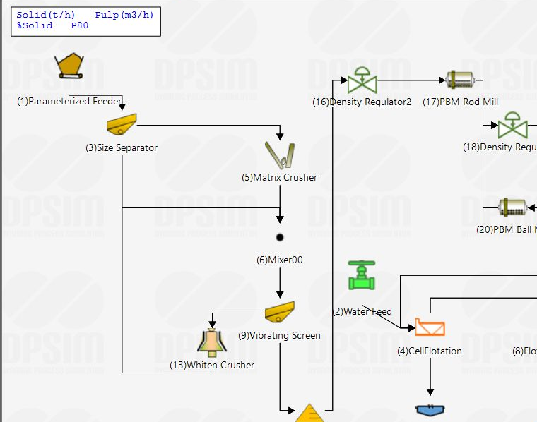 |
| Choose a free area near the feed. No connection is created when equipment is first placed. |
Figure 7. Canvas before adding the crusher.
| Canvas after adding the crusher |
|---|
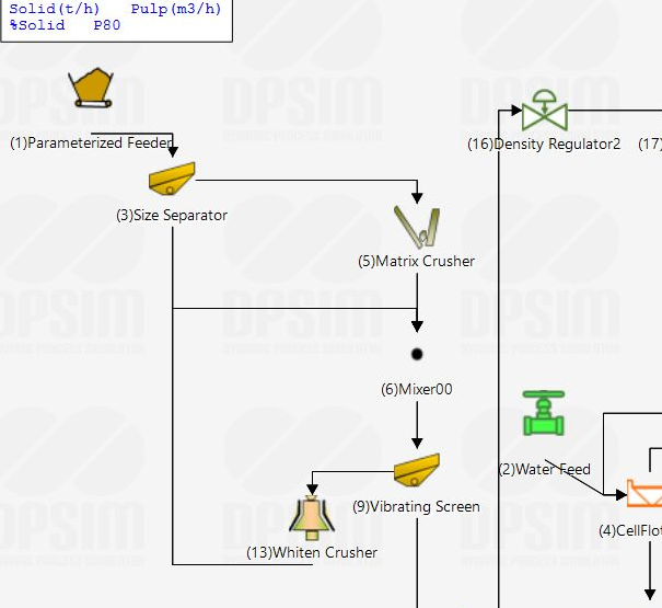 |
| The new crusher appears on the flowsheet with its equipment label. |
Figure 8. Same canvas after adding the crusher.
The new object is now part of the simulation project.
You can move it around the canvas to organize the flowsheet.
For the example we have been building throughout this series, position the crusher to the right of the feed:
Editable Feed → Crusher
Do not connect them yet.
We will create the material stream connections in the next tutorial.
| Feed and crusher positioned but not connected | Feed and crusher positioned but not connected | Feed and crusher positioned but not connected | Feed and crusher positioned but not connected | Feed and crusher positioned but not connected |
|---|---|---|---|---|
| Editable Feed | → | No material stream | → | Crusher |
| Source equipment | Position only | Process equipment |
Figure 9. Editable Feed and Crusher positioned beside each other but not connected.
Understanding equipment ports
When equipment is added to the flowsheet, it contains ports.
Ports define where material streams can enter or leave the equipment.
A simple unit may contain:
Feed port
and:
Product port
| Crusher material ports | Crusher material ports | Crusher material ports | Crusher material ports | Crusher material ports |
|---|---|---|---|---|
| Feed port | → | Crusher | → | Product port |
Figure 10. Simple equipment icon with Feed and Product ports identified.
An equipment model that produces two products may contain ports such as:
Feed
Oversize
Undersize
or:
Feed
Concentrate
Tail
depending on the operation.
| Screen material ports | Screen material ports | Screen material ports | Screen material ports | Screen material ports |
|---|---|---|---|---|
| Feed | → | Screen | → | Oversize |
| Screen | → | Undersize |
Figure 11. Screen with Feed, Oversize and Undersize ports.
The names of the ports are important because they represent the physical meaning of each material connection.
A screen, for example, does not simply produce two anonymous output streams.
One output represents the coarse product and the other the fine product.
Likewise, a flotation model may distinguish concentrate and tailings.
These port definitions become important when constructing more complex flowsheets.
One input does not always mean one stream
Some equipment can receive material from more than one upstream source.
A mixer is an obvious example.
Several incoming streams can be combined into a single output stream.
Conceptually:
Stream A + Stream B → Mixer → Combined Stream
| Mixer material ports | Mixer material ports | Mixer material ports | Mixer material ports | Mixer material ports |
|---|---|---|---|---|
| Stream A | → | Mixer | → | Combined product |
| Stream B | → | Mixer | ||
| Stream C | → | Mixer |
Figure 12. Mixer with multiple incoming streams and one output.
Other units may have multiple output ports.
For example:
Feed → Screen → Oversize + Undersize
or:
Feed → Separator → Concentrate + Tail
| Compare equipment port arrangements | Compare equipment port arrangements |
|---|---|
| One input / one output | One input / two outputs |
| • Crusher: Feed → Product | • Screen: Feed → Oversize + Undersize |
Figure 13. Examples of one-input/one-output and one-input/two-output equipment.
The process model defines what happens to the material between these ports.
Exploring the Classification category
Open:
Classification
The model library contains groups including:
Screens
Hydrocyclones
and:
Partition curves
| Classification model menu | Classification model menu | Classification model menu |
|---|---|---|
| Screens | Hydrocyclones | Partition curves |
| • Karra Screen • King Screen • Efficiency Screen | • Plitt Original • Plitt Modified Alpha | • Ideal Partition • Spline Partition |
Figure 14. Classification menu expanded.
The current library includes, among others, screen models such as Karra Screen and King Screen, as well as hydrocyclone and generic partition-curve approaches.
These models perform similar broad process functions — separating a particle population — but they do not necessarily calculate that separation in the same way.
A screen model may use equipment geometry and operating conditions.
A generic partition model may instead directly describe the probability of each particle size reporting to one product.
This illustrates why the model name matters.
Two icons representing classification equipment can correspond to fundamentally different mathematical assumptions.
Exploring Concentration and Dewatering
The Concentration category contains models that redistribute solid components between product streams.
Examples include flotation and component-recovery separators.
| Concentration model menu | Concentration model menu |
|---|---|
| Flotation | Separators |
| • King Flotation Cell • Finch Column Flotation | • Component Recovery • Three-parameter Recovery • Basic Separator |
Figure 15. Concentration menu expanded.
These models can change not only total mass distribution but also the composition of the resulting products.
For example:
Feed → Separation → Concentrate + Tailings
The valuable component may preferentially report to the concentrate while gangue preferentially reports to the tailings.
The Dewatering category contains models such as thickeners and filters.
| Dewatering model menu | Dewatering model menu | Dewatering model menu |
|---|---|---|
| Thickeners | Filters | Outputs |
| • Basic Thickener | • Basic Filter | • Underflow / Overflow • Cake / Filtrate |
Figure 16. Dewatering menu expanded.
These operations primarily redistribute solids and water between their products.
For example:
Thickener Feed → Underflow + Overflow
or:
Filter Feed → Cake + Filtrate
The same component and size representation that we defined earlier continues through these operations.
Auxiliary equipment
Not every object in a process flowsheet represents a major mineral processing transformation.
Flowsheets also require operations such as:
- mixing streams;
- dividing streams;
- representing intermediate storage;
- transporting material;
- applying simplified process constraints.
These functions are available under:
Auxiliary
| Auxiliary model menu | Auxiliary model menu | Auxiliary model menu |
|---|---|---|
| Routing | Buffers | Material handling |
| • Mixer • Two-output Splitter • Multi-output Splitter | • Static Pile • Dynamic Sump | • Slurry Pump • Open Launder |
Figure 17. Auxiliary menu expanded.
For example, a Mixer can combine several streams.
A Splitter can divide a stream between different process paths.
These units become particularly useful when constructing recycle circuits and more complex plant configurations.
Equipment icons are not the process model
The graphical icon helps communicate the flowsheet.
However, the icon should not be used to identify the model mathematically.
Two models may represent the same equipment family and therefore use similar or even identical graphical symbols.
| Similar symbols — different model names | Similar symbols — different model names | Similar symbols — different model names |
|---|---|---|
| Screen model 1 | Screen model 2 | Screen model 3 |
| • Karra Screen | • King Screen | • Efficiency Screen |
Figure 18. Similar equipment icons with different model names underneath.
When reviewing a simulation, always consider:
What equipment is this?
and separately:
Which model is calculating its behavior?
This distinction becomes especially important when comparing different modeling approaches for the same plant.
For example, two simulation cases could have visually identical crusher flowsheets while using different crusher models.
Their predicted results may therefore be different.
Naming equipment clearly
As the flowsheet grows, clear equipment labels become increasingly important.
A flowsheet containing labels such as:
Crusher 1
Crusher 2
Screen 1
may be sufficient for a tutorial.
For an engineering project, more descriptive identifiers are usually preferable.
Examples:
Primary Crusher
Secondary Screen
Ball Mill
Rougher Flotation
or project equipment tags such as:
CR-001
SC-001
BM-001
| Equipment labels on a DPSIM flowsheet |
|---|
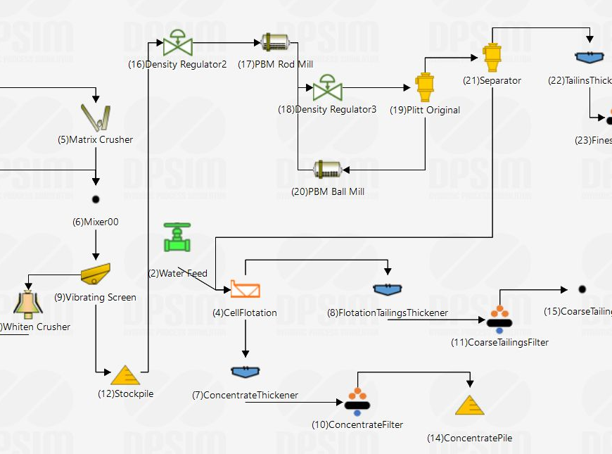 |
| Each graphical object keeps a visible equipment label below its symbol. |
Figure 19. Several units with clear equipment labels.
Good naming makes it easier to:
- read the flowsheet;
- identify equipment in results;
- compare simulation cases;
- export engineering data;
- communicate the model to other engineers.
The graphical flowsheet should remain understandable even to someone who did not build it.
Selecting a model is an engineering decision
Adding equipment to the canvas is easy.
Choosing the correct model requires more thought.
Before selecting a model, consider what information you actually have.
For example, suppose you need to simulate a crusher.
You may have:
- only a known product PSD;
- CSS and general operating information;
- detailed plant survey data;
- equipment-specific information;
- calibrated breakage parameters.
These different data sets may justify different modeling approaches.
| Match model complexity to available information | Match model complexity to available information | Match model complexity to available information | Match model complexity to available information | Match model complexity to available information |
|---|---|---|---|---|
| Available data | → | Appropriate model complexity | → | Reliable result |
| Measured inputs | Engineering choice | Defensible prediction |
Figure 20. Data Available → Appropriate Model Complexity.
This principle applies throughout the DPSIM library.
Model selection should therefore follow the engineering question rather than the desire to use the most detailed model available.
Model parameters come next
Once an equipment model has been added, it normally requires parameters before its behavior is fully defined.
Depending on the selected model, these parameters might include quantities such as:
- equipment dimensions;
- operating settings;
- partition parameters;
- water split;
- recovery;
- residence time;
- specific energy;
- power;
- material-dependent parameters.
We will explore the equipment editing interface in detail later.
For now, leave the newly added equipment with its default parameters.
Our immediate objective is to construct the flowsheet topology first.
Building the first process sequence
Using the material feed created in the previous tutorial, add one process equipment item beside it.
For example:
Editable Feed
followed by:
Crusher
The canvas should now contain two separate objects:
Editable Feed Crusher
| Place the feed and crusher in sequence | Place the feed and crusher in sequence | Place the feed and crusher in sequence | Place the feed and crusher in sequence | Place the feed and crusher in sequence |
|---|---|---|---|---|
| Editable Feed | → | Position in process order | → | Crusher |
| Source equipment | No stream yet | Process equipment |
Figure 21. Editable Feed and Crusher positioned in sequence.
At this point, they are only positioned next to each other.
There is still no material connection between them.
DPSIM does not infer process connectivity from the graphical position of equipment.
Placing a crusher beside a feed does not mean that the crusher receives that feed.
The units must be explicitly connected through a stream.
This distinction is fundamental:
Position defines the drawing.
Streams define the process connectivity.
What we have established
The project now contains:
Material definition
Components, size classes, flowrates, PSD and composition.
And:
Process equipment
A model-backed unit placed on the flowsheet.
The next step is to connect these elements so that material can move through the process model.
In the next tutorial, we will create material streams, connect equipment ports and begin building the actual flowsheet network.
We will also see how DPSIM distinguishes the origin and destination of each stream and why connection direction matters.
| Completed material connection | Completed material connection | Completed material connection | Completed material connection | Completed material connection |
|---|---|---|---|---|
| Editable Feed | → | Material stream | → | Crusher |
| Product port | Direction of flow | Feed port |
Figure 22. Preview showing Feed connected to Crusher by a stream.