We have already defined two fundamental properties of our DPSIM project:
Components define what the solid material contains.
Size classes define how the particle population is divided by size.
Now we can create the material that actually enters the flowsheet.
In DPSIM, this can be done using an Editable Product Stream Feed, which creates a source stream whose flowrate, particle size distribution and component composition can be defined directly by the user.
In this tutorial, we will build our first complete material stream.
In this tutorial you will learn how to:
- add an Editable Product Stream Feed;
- understand the relationship between the feed equipment and its output stream;
- define dry solids and water flowrates;
- enter a particle size distribution;
- define component composition by particle size;
- understand how DPSIM calculates the overall component grades.
Adding an Editable Product Stream Feed
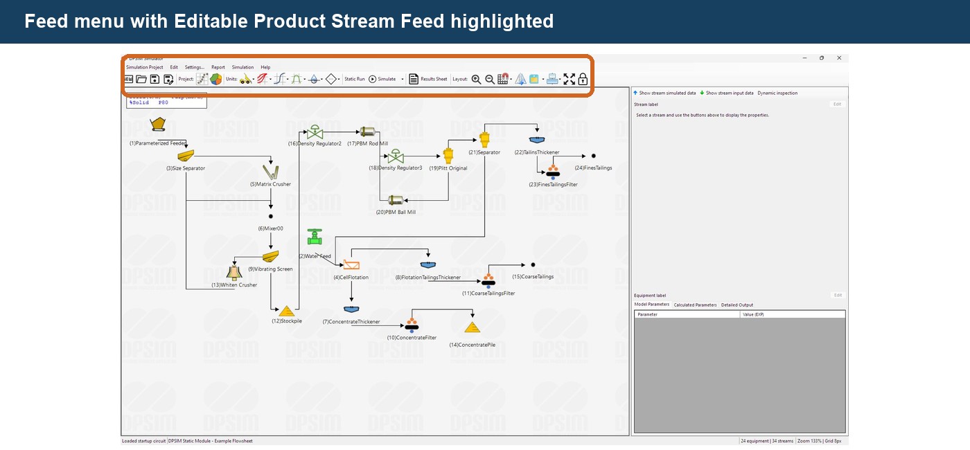
From the DPSIM toolbar, open:
Feed → Editable Product Stream Feed
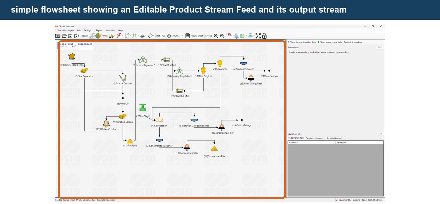
Add the feed to the flowsheet canvas.
The new object represents a material source entering the simulation.
Unlike process equipment such as a crusher or screen, the feed does not transform an incoming material.
It has no process feed stream.
Instead, it creates a single output stream that defines the material entering the flowsheet.
Conceptually:
User-defined material → Feed → Process flowsheet
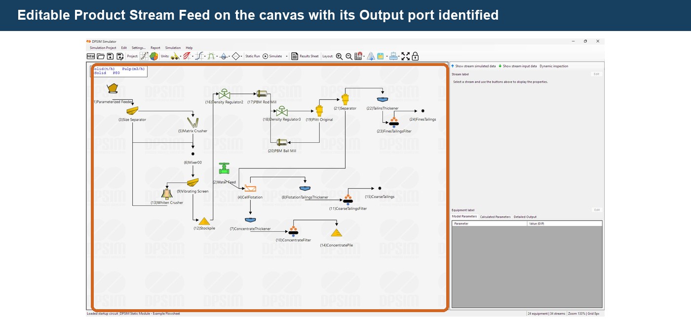
The default flowsheet label is Editable Feed Stream, and the generated material stream is initially named Feed.
These labels can be changed to something more representative of the study, such as:
ROM Feed
Grinding Feed
Flotation Feed
or:
Sample A
The feed data belong to the stream
This is an important DPSIM concept.
The feed icon identifies the source, but material properties such as flowrate, particle size distribution and composition belong to its output stream.
The Editable Product Stream Feed itself does not contain a set of process model parameters.
Instead, you define the material directly on the stream.
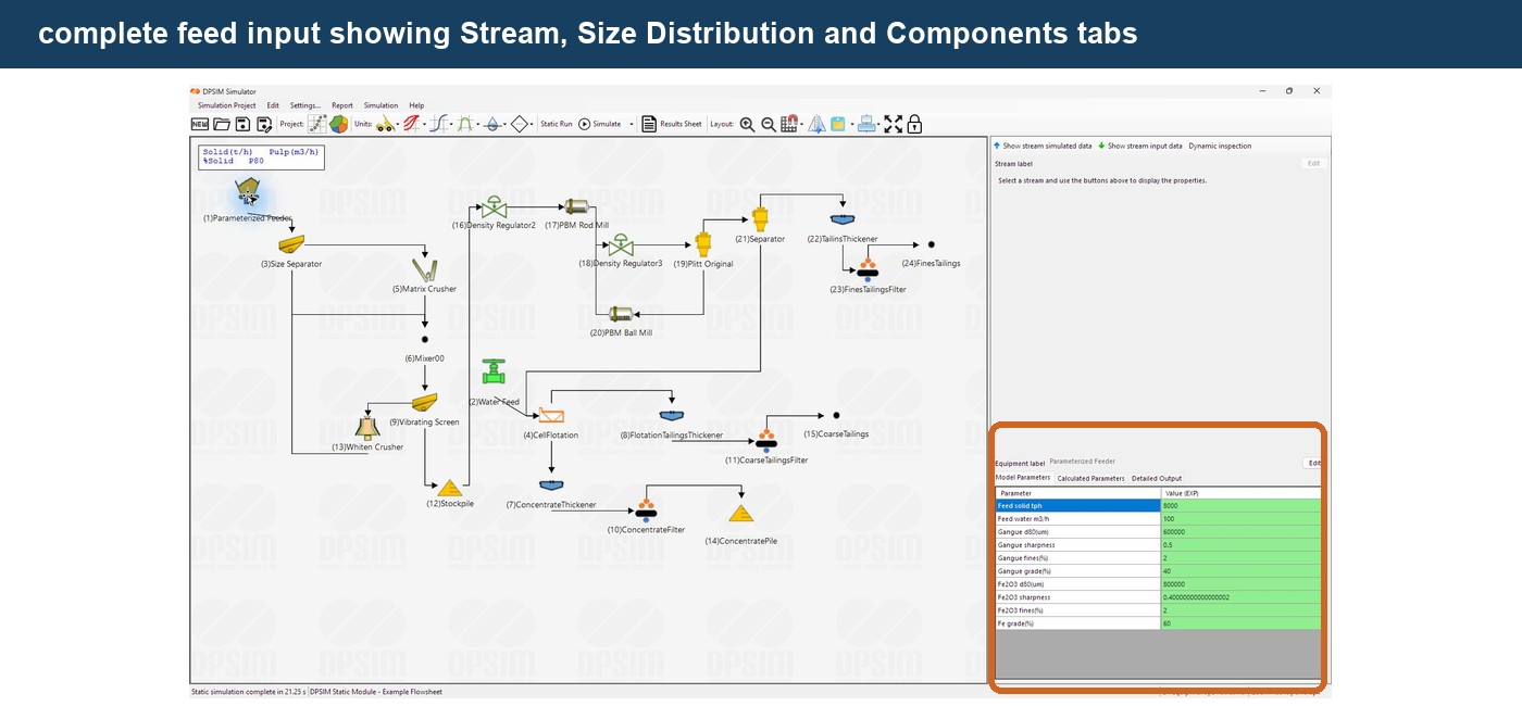
Once the feed stream is connected and visible on the flowsheet, select the stream and choose:
Show stream input data
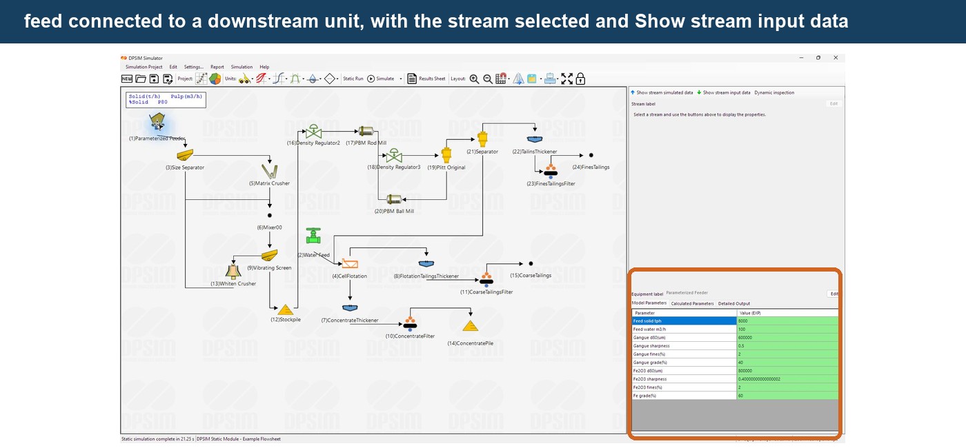
The stream input area contains three main tabs:
Stream
Size Distribution
Components
These three sections describe the material entering the simulation.
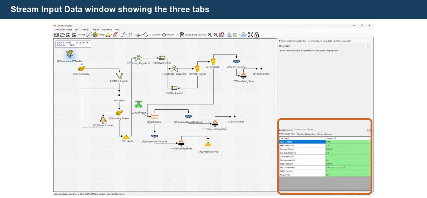
We will configure each of them separately.
Defining the material flowrate
Open the:
Stream
tab.
Two input quantities are available:
Solid flowrate
and
Water flowrate
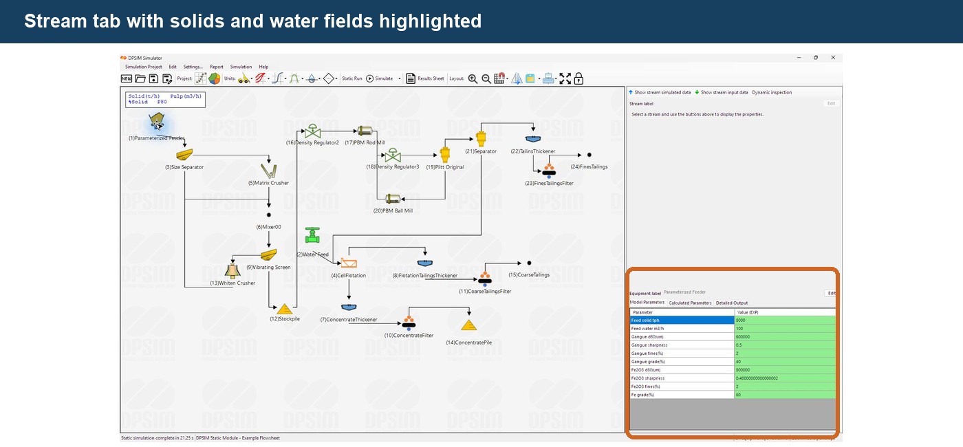
The solids flowrate represents the dry solid mass entering the simulation.
For example:
Dry solids = 1,000 t/h
The water flow represents the water associated with the material.
For a dry crushing circuit, this value may be zero or relatively small.
For a grinding or beneficiation circuit, the feed may already be a slurry and contain a significant amount of water.
For example:
Dry solids = 1,000 t/h
Water = 600 t/h
DPSIM uses these values together with the material properties to calculate other stream quantities later, including percent solids, slurry density and volumetric flowrate.
Engineering note
Whenever possible, define the feed using independent measured quantities.
For example, if dry solids flowrate and percent solids are known from plant data, calculate the corresponding water flow before entering the stream.
Avoid independently specifying several quantities that describe the same mass balance unless they are internally consistent.
Entering the particle size distribution
Open the:
Size Distribution
tab.
The size classes previously defined for the project will appear automatically.
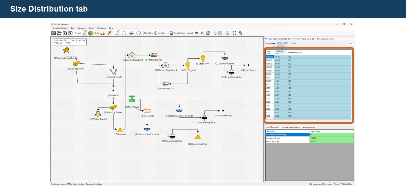
The table contains the project particle sizes together with:
% Retained (EXP)
The PSD is therefore entered as fraction retained in each size class.
For example:
| Size | % Retained |
|---|---|
| 1000 µm | calculated |
| 500 µm | 10 |
| 250 µm | 25 |
| 125 µm | 30 |
| 63 µm | 20 |
| 38 µm | 10 |
| Pan | calculated |
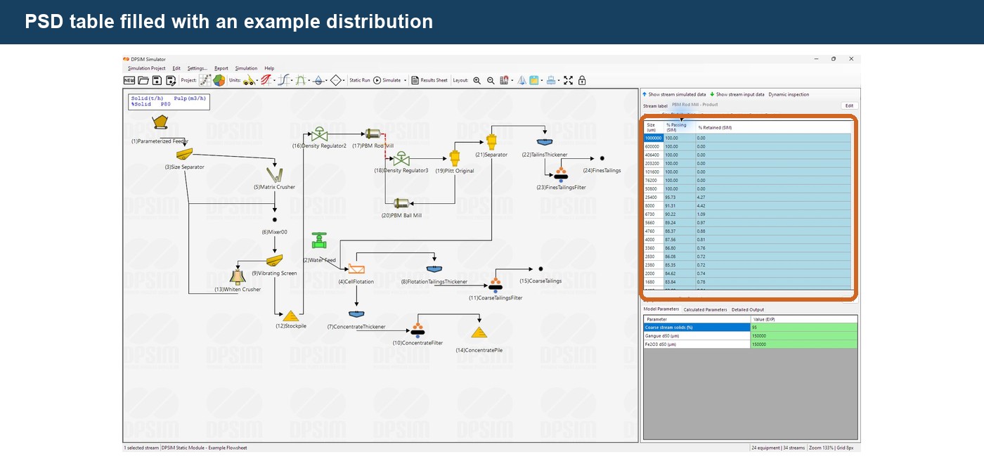
Remember the convention established in the previous tutorial:
DPSIM stores the particle size classes in descending order.
The coarsest size is at the top of the table and the finest fraction is at the bottom.
The top-size and pan rows
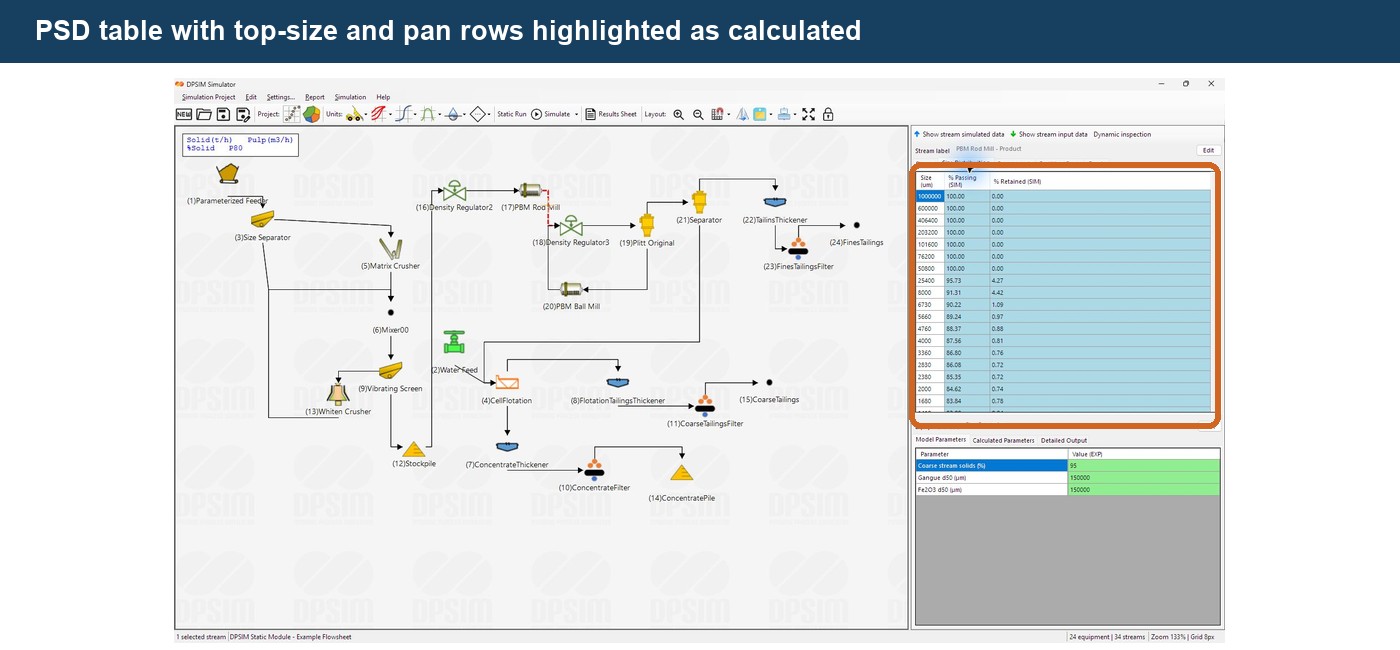
Two PSD rows are handled automatically by DPSIM.
The top-size row is not directly edited.
Its retained fraction is zero because it represents the upper boundary of the particle population.
The pan fraction is also calculated automatically.
DPSIM calculates the pan as the remainder required for the complete retained distribution to equal 100%.
Conceptually:
Pan = 100% − Sum of the editable retained fractions
For example, if the editable fractions total:
92%
then DPSIM assigns:
Pan = 8%
The editable retained fractions cannot total more than 100%.
This makes it unnecessary to manually close the PSD balance.
Retained and passing distributions
Laboratory PSD data are often reported as cumulative percent passing, while the DPSIM input table uses percent retained by size class.
These are two representations of the same particle size distribution.
For example, suppose the cumulative passing data are:
| Size | % Passing |
|---|---|
| 500 µm | 90 |
| 250 µm | 65 |
| 125 µm | 35 |
| 63 µm | 15 |
The retained fraction between 500 and 250 µm is obtained from the difference between consecutive passing values:
90 − 65 = 25%
Likewise, between 250 and 125 µm:
65 − 35 = 30%
The general relationship is:
Retained in a size interval = Passing at the upper size − Passing at the lower size
Once the retained fractions are entered, DPSIM can reconstruct the cumulative passing curve.
Pasting PSD data from Excel
The stream input grids support copying and pasting data from the clipboard.
This is useful when laboratory sieve results are already available in Excel.
Prepare the retained percentages in the same order as the DPSIM size mesh:
largest → smallest
Copy the values from Excel and paste them into the editable PSD cells using:
Ctrl + V
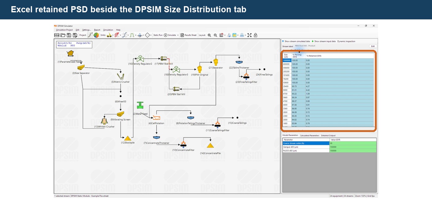
This can be much faster than entering a long size distribution manually.
Before pasting, always verify:
- the size classes match the DPSIM project mesh;
- the order is descending;
- the values are retained percentages;
- the total does not exceed 100%.
Defining component composition
The PSD tells us how much solid is present in each size class.
We still need to define what that solid contains.
Open the:
Components
tab.
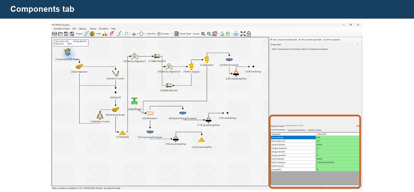
The first column contains the particle sizes.
Each additional column represents one of the components previously defined for the project.
For example:
| Size | Hematite | Quartz |
|---|---|---|
| 500 µm | 70% | 30% |
| 250 µm | 75% | 25% |
| 125 µm | 80% | 20% |
| 63 µm | 85% | 15% |
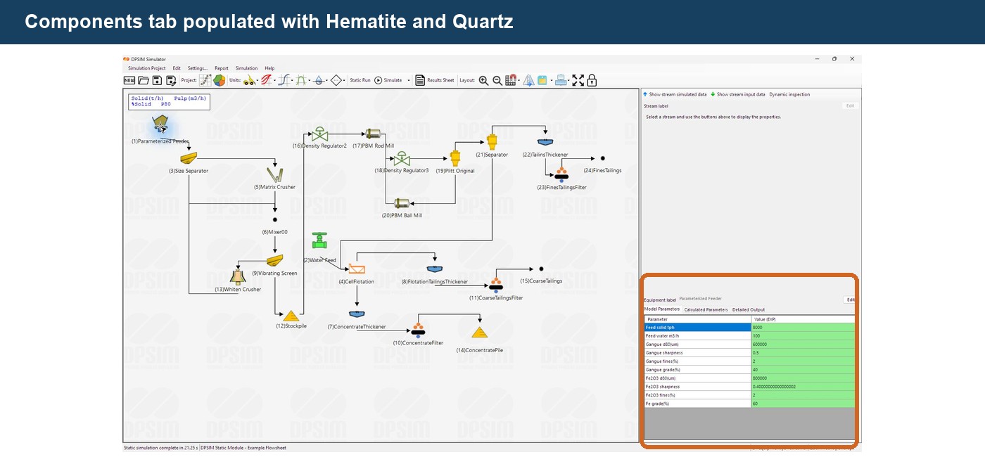
Each row describes the composition of the solids within that particular particle size class.
This is different from the PSD.
The PSD answers:
How much material is in this size class?
The component table answers:
What is that material made of?
Together, the two tables completely describe the solid particle population.
Component-by-size composition
Consider a feed containing two components:
Hematite
and
Quartz
Suppose that 25% of the total feed mass is retained in one particular size interval.
If that size class contains:
80% Hematite
and:
20% Quartz
then the contribution of that size interval to the total stream is:
Hematite = 25% × 80% = 20% of total solids
Quartz = 25% × 20% = 5% of total solids
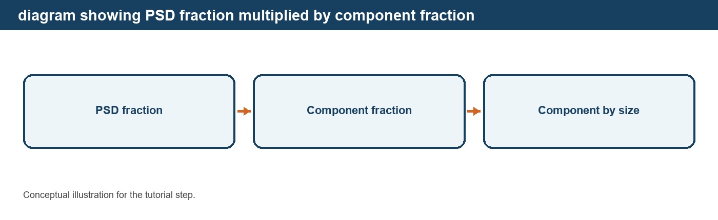
DPSIM performs this relationship across all particle size classes.
The result is a complete component-by-size mass distribution.
This representation is fundamental because many mineral processing operations do not affect every component and every particle size in the same way.
Components in each size class must close
For a complete component representation, the fractions within each size class should add to:
100%
For example:
Hematite 75% + Quartz 25% = 100%
DPSIM prevents the entered component composition in a size class from exceeding 100%.
If three components are used:
Hematite = 70%
Quartz = 20%
Kaolinite = 10%
then:
70 + 20 + 10 = 100%
This represents the complete solid composition of that particle size class.
Overall grade is calculated from the size-by-size composition
One important consequence of the DPSIM material structure is that the overall component grade does not need to be independently specified when the complete size-by-size composition is known.
DPSIM combines:
the mass retained in each particle size class
with:
the component fraction within that class
to calculate the overall stream composition.
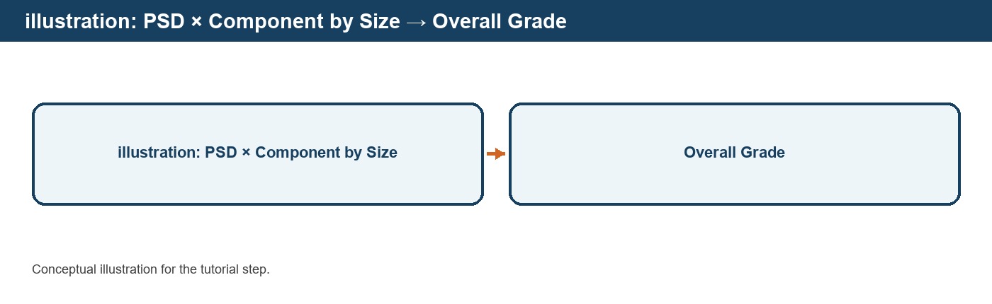
For component (c), conceptually:
Overall grade = Σ(Size fraction × Component fraction in that size)
This is useful because the model preserves information that a single global assay would lose.
Two feeds could have the same overall Fe grade while having very different Fe distributions by particle size.
Those two materials could behave very differently in a classifier, magnetic separator, flotation circuit or other size-dependent process.
Example: building a complete feed description
Suppose our project contains:
Hematite
Quartz
and the size mesh:
1000 → 500 → 250 → 125 → 63 → 38 µm → Pan
We define:
Dry solids: 1,000 t/h
Water: 500 t/h
Then we enter the feed PSD:
| Size | Retained |
|---|---|
| 1000 µm | calculated |
| 500 µm | 8% |
| 250 µm | 22% |
| 125 µm | 30% |
| 63 µm | 20% |
| 38 µm | 12% |
| Pan | calculated |
The editable classes total:
92%
so DPSIM calculates:
Pan = 8%
Now suppose the hematite content becomes progressively higher toward the finer fractions.
The Components tab might contain:
| Size | Hematite | Quartz |
|---|---|---|
| 1000 µm | 60% | 40% |
| 500 µm | 65% | 35% |
| 250 µm | 70% | 30% |
| 125 µm | 75% | 25% |
| 63 µm | 80% | 20% |
| 38 µm | 85% | 15% |
| Pan | 90% | 10% |
The feed is now much more than a single number such as:
1,000 t/h at 72% Fe-bearing material
DPSIM knows how the material mass and composition are distributed across the particle size range.
Why component-by-size data matter
A global assay can be sufficient for simple overall mass balances.
But many mineral processing models require a more detailed description.
Consider a feed where the valuable component is concentrated in the fine fraction.
A screen separating coarse and fine particles will then also change the grade of its products, even though the screen itself does not explicitly separate minerals.
The same principle applies to classification.
If mineral composition varies with particle size, then:
size separation also becomes component separation.
This is one of the reasons particle population models are powerful in mineral processing simulation.
They allow the simulator to preserve the interaction between:
mass
particle size
and
composition
throughout the flowsheet.
Feed data should reflect the available information
Not every project will have component-by-size assays.
Sometimes only the bulk grade and bulk PSD are available.
In that case, the model should not imply a level of knowledge that the data do not support.
One possible simplifying assumption is to use the same component composition for every particle size class.
For example:
Hematite = 75% at all sizes
Quartz = 25% at all sizes
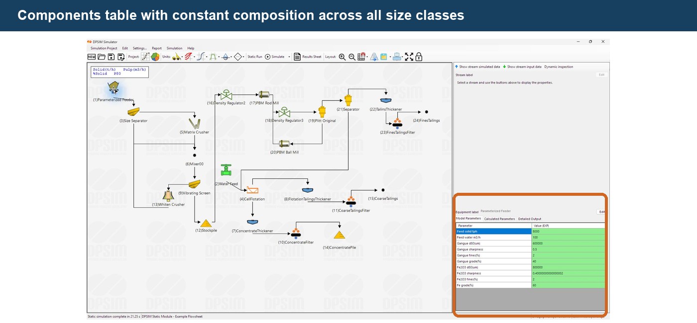
This means that the component PSDs initially follow the same shape as the bulk PSD.
It is a simplification, but it is explicit and internally consistent.
If size-by-size assay data become available later, the feed description can be refined.
Engineering note
The objective is not to populate every available DPSIM field with different numbers.
The objective is to represent the material using the best information actually available.
Checking the feed before continuing
Before moving on, verify the following:
- dry solids flowrate is correct;
- water flowrate is correct;
- PSD corresponds to the selected project size mesh;
- retained fractions do not exceed 100%;
- the automatically calculated pan is reasonable;
- component composition is physically consistent;
- component fractions in each size class represent the complete solids;
- component names and densities correspond to the project definition.
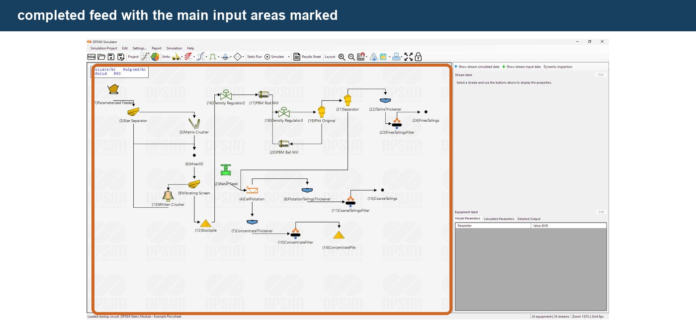
At this point, the DPSIM project contains its first fully characterized material stream.
We now know:
how much material enters
how much water enters
how the solids are distributed by size
and
what the solids contain at each size
From material definition to process flowsheet
So far, we have concentrated on the material itself.
The next step is to begin constructing the process that will treat it.
DPSIM contains different equipment families representing operations such as:
- crushing;
- grinding;
- screening;
- classification;
- flotation;
- magnetic separation;
- gravity separation;
- thickening;
- filtration;
- auxiliary process operations.
Each equipment object can contain a mathematical model that determines how the incoming stream is transformed into one or more product streams.
In the next tutorial, we will explore the DPSIM equipment library and learn how process units and models are added to the flowsheet.