
Player · Tutorial
From recorded samples to an analysis
A trend, a histogram and a CSV describe the same recorded series in different ways. A small interval makes their relationship visible and checkable.
A trend describes sequence; a histogram describes frequency
A time trend retains the order of observations. It helps explain when a change occurred and how one quantity varied alongside another. A histogram groups values into bins and counts their occurrences. It describes the distribution of the selected samples while leaving their temporal order aside.
A CSV retains the recorded rows as text for independent analysis. Comparing these three representations is useful because a graph’s appearance alone does not establish its sample count, population or numerical summary. In this lesson the 40–80 s interval supplies five known instants. These numerical values belong to the recording shown in the screenshots. For another recording, use its own samples: the check is that the chart, histogram and CSV agree for the same variable and interval, not that they reproduce this example's random values.
Two quantities can follow the same shape with different units
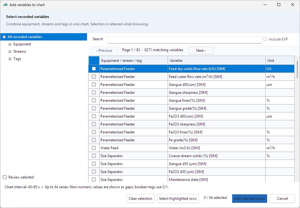
The selected equipment and variable identify what a curve represents. In the practice file, feeder dry-solids flow is measured in t/h and water flow in m³/h. The ROM logic relates the commands by a factor of 0.01; the units and physical meanings remain different.
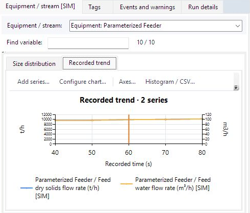
The two curves can overlap when the two Y axes have corresponding scales. That overlap follows from the fixed relationship, not from equality of the two numerical values. At 60 seconds the file contains about 9,950.1046 t/h dry solids and 99.5010 m³/h water.
Exercise: relate the plotted curves to their definitions
- Select the 40–80 s analysis interval and open Recorded trend. In Add series, find the Parameterized Feeder’s dry-solids and water-flow variables and check both entries.
- Confirm the selected-variable count before adding them. A highlighted row and a checked row have different meanings in the picker; Review selected shows the retained selection.
- Read the legend and both Y-axis units. Compare the two values at 60 seconds and calculate their ratio.
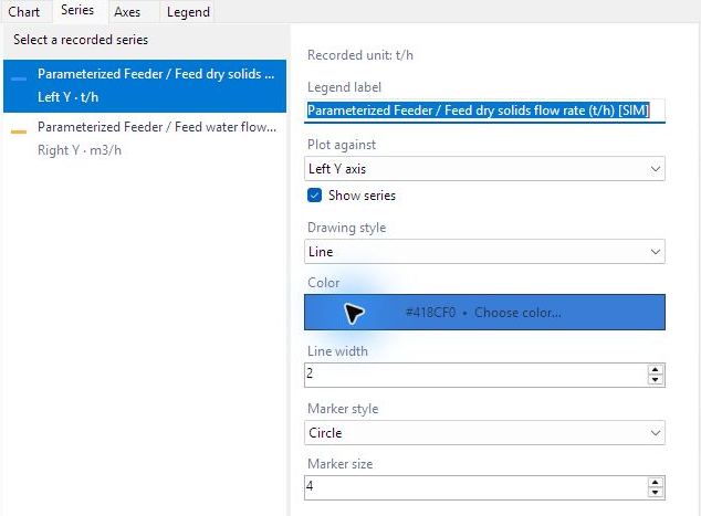
- Use Edit chart on the displayed chart, or Edit selected chart in Chart studio, to inspect the selected series and its axis assignment without changing its recorded unit.
The interval defines the population to be analyzed
A chart kept in the library has its own saved interval. In Chart library, select the time chart, open Time range, check the time unit and the inclusive From and To values, then choose Update all series. This reads the selected recording samples for every series while retaining the chart appearance. Changing only the visible axis limits would crop the drawing without choosing a new population of recorded data.
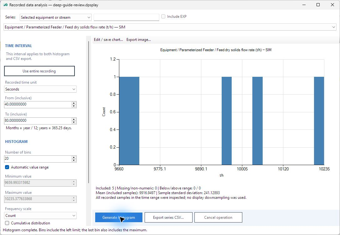
For the inclusive 40–80 s interval, the practice file has five dry-solids values. Automatic histogram limits include all five. A manual value range could exclude some, so the included, missing and out-of-range counts are part of the interpretation, not secondary status information.
| Recorded time (s) | Dry solids (t/h) |
|---|---|
| 40 | 9,659.99331598 |
| 50 | 9,697.04827140 |
| 60 | 9,950.10464757 |
| 70 | 10,042.22466817 |
| 80 | 10,235.37763387 |

Their arithmetic mean is 9,916.9497074 t/h and their sample standard deviation is 241.1289276 t/h. The latter uses n − 1 in the denominator. These describe the included samples; they do not by themselves quantify uncertainty in the process model. Five samples are enough to check this procedure, but not to establish a reliable long-run probability distribution.
Exercise: account for every sample
- Open Analysis and select the feeder dry-solids series. Confirm the inclusive From and To values of 40 and 80 seconds.
- Generate a histogram with automatic value range. Compare the included count with the five instants derived from the recording cadence.
- Read the missing/non-numeric and outside-range counts before interpreting the mean. In the captured file both are zero.
- Consider what would happen if manual value limits excluded the largest value. The histogram’s included population would change even though the recording itself had not.
The CSV provides an independent numerical check
The verified export used a semicolon separator and decimal comma. It contained one header and the five recorded rows:
Time (s);Feed solid tph [SIM] (t/h)
40;9659,9933159817101
50;9697,0482713995098
60;9950,1046475722505
70;10042,224668172301
80;10235,3776338676
Export series CSV uses all recorded rows in the chosen time range, including missing values. It does not merely copy the points retained for chart display. If manual histogram value limits exclude a sample, the CSV and histogram can legitimately have different populations.
For an independent check, the separator and decimal convention must be interpreted correctly by the receiving application. The exported five rows reproduce the Player mean and sample standard deviation. A single-column import indicates a delimiter mismatch; text-valued numbers often indicate a decimal-convention mismatch.
The analysis reference documents the controls. The following lesson explains how the resulting charts and interval can be kept with the recording.