
Player · Tutorial
Recorded time and analysis intervals
The state currently shown, the data interval being analyzed and the visible timeline window are related, but they are not the same selection.
Three different questions about time
| Question | Selection in the example | Meaning |
|---|---|---|
| What did the process look like then? | Recorded state at 60 s, state 7/13 | The instant whose values are shown in the route and inspector. |
| Which data are being compared? | Analysis interval 40–80 s | The saved samples included in trends, histograms and CSV analysis. |
| Which part of the time axis is visible? | Timeline window 0–120 s | The part of the sequence currently in view. |

Moving the playhead changes the current process state. Changing the analysis interval chooses a population of samples. Zooming the timeline changes its visible window. Keeping these questions separate explains why selecting an interval does not automatically move the current process instant.
A saved sequence has discrete instants

Green markers correspond to recorded states; grey markers correspond to calculated cycles without saved values. Seeking between saved instants displays the recorded state at or before the requested time. The Recorded time label identifies what actually loaded, which can differ from the location originally requested.
Playback speed changes the rate at which this saved sequence is presented. It does not change the calculation step used by the producing run or insert newly calculated states. If a transient occurred between saved instants, a closer timeline zoom cannot recover it.
Exercise: observe one instant and select an interval
- With the practice recording open, expand the timeline, select Seconds as the display unit and use Show all. Locate the 60-second region.
- Select that region and wait for the state to load. The practice file reports Recorded time: 60 s / 120 s (7/13). Compare a selected item with its preceding recorded state.
- Set the Analysis range to 40 and 80 seconds, finishing each field edit. The blue selection should span those endpoints while the current process state can remain at 60 seconds.
- Use Fit selection to view the chosen region more closely, then Show all to restore the full time axis. The analysis range should remain the same.
Time also qualifies the inspector’s values
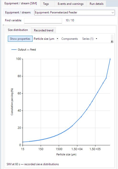
The inspector follows the selected owner and current recorded state. A stream size-distribution curve therefore describes that stream at one saved instant, while a Recorded trend describes a quantity across an interval. Switching between those plots changes the question being asked.
SIM identifies simulation output. EXP identifies experimental/input data when it was supplied to the recording. Absence of EXP is not a zero-valued measurement. Likewise, a variable hidden by the inspector’s search filter is different from a variable absent from the file.
The µm/mm control changes the displayed aperture unit. The owner, port, units and recorded time remain necessary to interpret the curve. Show properties and Expand chart change the available viewing space; their documented behavior is in the inspector reference.
Why the distinction matters when reopening a review
A saved presentation can retain an analysis interval and chart library even if the playhead starts at zero when reopened. This does not contradict interval persistence: one selection defines the data being analyzed, while the other defines the instant currently displayed. The next lesson uses the five-sample interval to connect these time concepts to numerical analysis.