How study logic changes the process

A tag is the connection between logic and model

The equipment model already contains an input for feeder dry-solids flow. The script does not implement the feeder model again. Instead, it calculates a command and writes it through a tag bound to that input. A tag therefore gives study logic a named access point to a model quantity.

The name identifies the tag in the script, while its type, target and selected parameter define its behavior. An Internal value has no automatic equipment connection. A read binding exposes a value for inspection; a write binding permits an assignment to an exposed editable input.

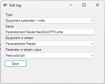
In this binding, the target is Parameterized Feeder and the parameter is Feed solid tph. The .write suffix helps a reader recognize the naming convention, but the actual binding configuration governs the write. The water command has a separate binding to Feed water m3/h.

Why execution order matters

A calculation cycle can contain more than one statement about the same input. The normal feed script may propose a positive rate, while an availability interlock later replaces it with zero. The sequence determines which command reaches the calculation.

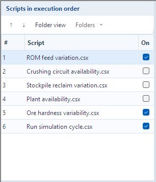
The captured example enables ROM variation, ore parameter variation and the cycle request. The other scripts are present but disabled. Selecting a script displays its source; it does not enable it. Folder grouping is authoring organization and does not replace the global execution order.

The individual controls are described in the script reference. Here the important relationship is that normal commands precede the interlocks that may override them, and the supplied cycle request follows the command logic.

The ROM script as a mathematical model of a disturbance

The example represents a changing feed with a bounded random walk. At each calculation cycle it adds a small signed increment to the current command, then restricts the result to a permitted band. This differs from selecting a completely new independent value anywhere in the band at each cycle.

// Smooth random variation of the run-of-mine (ROM) feed.
// Solids rate: t/h. Water flow: m^3/h. Preserve the nominal water-to-solids ratio.
// Total variation: +/-20%; maximum change per cycle: +/-1% of nominal.

if (!IsDynamic)
    return;

double nominalSolidsRate = 10000.0;
double nominalWaterFlow = 100.0;
double variationFraction = 0.20;
double cycleVariationFraction = 0.01;

string solidsRateTag =
    "Parameterized Feeder.feedSolidTPH.write";

string waterFlowTag =
    "Parameterized Feeder.feedWaterM3PH.write";

double minimumRate = nominalSolidsRate * (1.0 - variationFraction);
double maximumRate = nominalSolidsRate * (1.0 + variationFraction);

double currentRate = Tags.GetNumber(solidsRateTag);

if (currentRate <= 0.0)
    currentRate = nominalSolidsRate;

var random = new System.Random();

double increment = nominalSolidsRate * cycleVariationFraction
                  * (2.0 * random.NextDouble() - 1.0);

double newRate = currentRate + increment;

newRate = System.Math.Max(minimumRate, newRate);
newRate = System.Math.Min(maximumRate, newRate);

double newWaterFlow = nominalWaterFlow * newRate / nominalSolidsRate;

Tags.SetNumber(solidsRateTag, newRate);
Tags.SetNumber(waterFlowTag, newWaterFlow);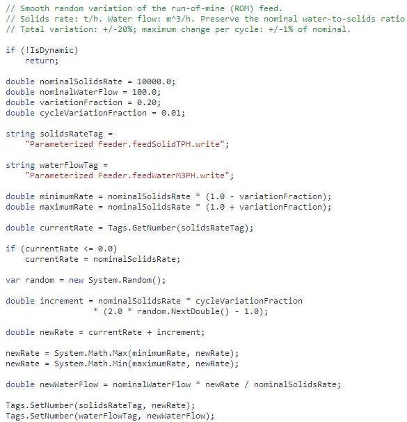

Following the calculation from input to command

A. Dynamic execution context

if (!IsDynamic) return; prevents this study logic from being applied in another execution mode. It does not start the simulator. The local steady-state check already excludes dynamic scripts.

B. Reference values and relative bounds

For example, if the current command is 10,000 t/h and the random draw is 0.75, the increment is 10,000 × 0.01 × (2 × 0.75 − 1) = 50 t/h. The next solids command is 10,050 t/h and water is 100.5 m³/h. If the tentative solids command exceeds 12,000 or falls below 8,000, the two Math calls clip it to the band.

C. Names and bindings

The two strings must match the existing Tags catalog exactly. The solids name binds to Feed solid tph; the water name binds to Feed water m3/h. The script does not search the flowsheet for a similarly named equipment item.

D. Current command and initialization

Tags.GetNumber(solidsRateTag) reads the bound numeric command. A value at or below zero is replaced in the local calculation by the nominal reference. That fallback is relevant when an earlier stop left the command at zero; it is not a check that every other input is physically valid.

E. The random increment

NextDouble produces a draw from zero up to, but not including, one. Scaling it to 2u − 1 produces a signed increment. Adding that increment to the current command gives a walk from the preceding command rather than a new independent draw from 8,000–12,000.

F. Bounds and clipping

Math.Max applies the lower bound and Math.Min applies the upper bound. A tentative 12,040 t/h is clipped to 12,000 t/h; a tentative 7,970 t/h is clipped to 8,000 t/h. Clipping can accumulate values at a boundary, so the resulting distribution need not be uniform.

G. Water ratio and command writes

The ratio calculation gives the water command in m³/h from a dry-solids command in t/h. The final two SetNumber calls write the targets. These are parameter commands: actual stream output follows the selected model, current state and any later override.

Exercise: predict one cycle before running it

1. In the example copy, inspect the solids and water tags and confirm their target parameters and units. The script strings should match the catalog names exactly.
2. Select ROM feed variation and compare its nominal values with the feeder’s saved inputs. These have different roles: the saved input supplies a starting command, while the nominal value defines the script’s reference band and step size.
3. Without changing the code, calculate the result for a current command of 10,000 t/h and a random draw of 0.75. Then consider a tentative command of 12,040 t/h before clipping.
4. Review the enabled state and order of the crushing interlock. Consider what happens if it runs after the normal command and finds an unavailable item.

What a recorded curve can establish

A successful run can be examined in Player by plotting the feeder commands and the actual stream outputs. With only the normal ROM writer affecting the two feed commands, water follows solids × 0.01. Actual downstream delivery can differ because equipment behavior, storage and later overrides intervene.

The random object has no explicit repeatability seed, so separate runs need not reproduce the same sequence. Changing the calculation step also changes the number of random updates per simulated hour. The useful checks are the bounds, units, relationships and order, rather than an expectation of matching a screenshot point for point.

The worked example with all six scripts continues this reasoning through reclaim behavior, availability interlocks, the illustrative ore parameter settings and Runner’s cycle-advancement rule. Compilation and execution occur in Runner; a successful preflight does not prove the script will run successfully.